Stylometry and the Voice of Hildegard#

Introduction#

Hildegard of Bingen, sometimes called the “Sybil of the Rhine”, was a famous author of Latin prose in the twelfth century. Female authors were a rarity throughout the Middle Ages and her vast body of mystical writings has been the subject of numerous studies. Her epistolary corpus of letters was recently investigated in a stylometric paper focusing on the authenticity of a number of dubious letters traditionally attributed to Hildegard [Kestemont et al., 2015]. For this purpose, Hildegard’s letters were compared with that of two well-known contemporary epistolary oeuvres: that of Bernard of Clairvaux, an influential thinker, and Guibert of Gembloux, her last secretary. Fig. 16 (reproduced from the original paper) provides a bird’s eye visualization of the differences in writing style between these three oeuvres. Documents written by Hildegard, Bernard of Clairvaux, and Guibert of Gembloux are assigned the prefixes H_, B_, and G_ respectively. The words printed in gray show which specific words can be thought of as characteristic for each author’s writing style. As can be gleaned from the scatter plot in the left of the panel, these oeuvres fall into three remarkably clear clusters for each author, suggesting that the three authors employed markedly distinct writing styles.

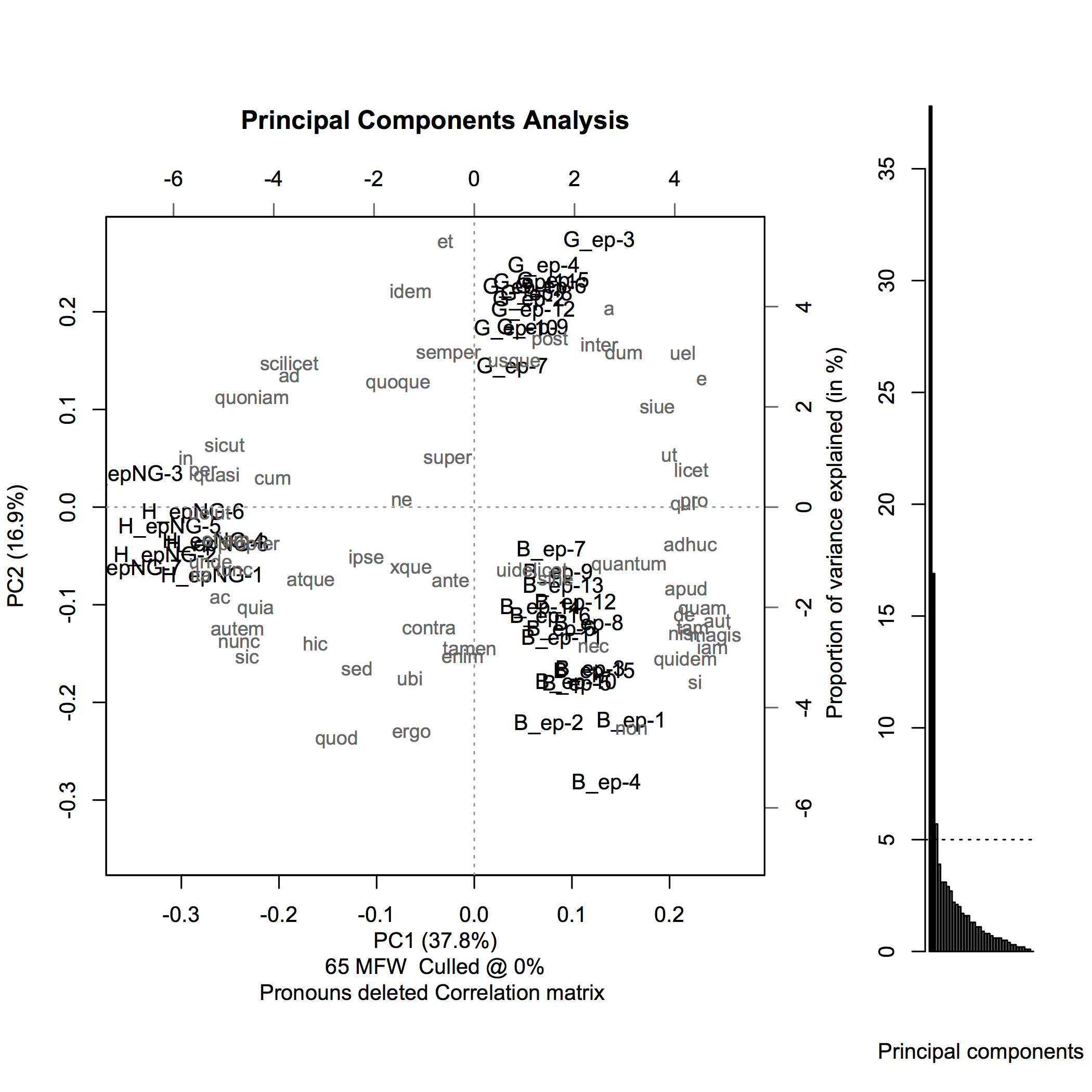
Fig. 16 A Principal Component Analysis (PCA) plot (first 2 dimensions) contrasting 10,000 lemmatized word samples from three oeuvres (Bernard of Clairvaux, Hildegard of Bingen, and Guibert of Gembloux). After Kestemont et al. [2015].#

The goal of this chapter is to reproduce (parts of) the stylometric analysis reported in Kestemont et al. [2015]. While chapter Introduction to Probability already briefly touched upon the topic of computational stylometry, the current chapter provides a more detailed and thorough overview of the essentials of quantitatively modeling the writing style of documents [Holmes, 1994, Holmes, 1998]. This has been a significant topic in the computational humanities and it continues to attract much attention in this field [Siemens and Schreibman, 2008]. Stylometry is typically concerned with modeling the writing style of documents in relation to, or even as a function of, metadata about these documents (cf. Herrmann et al. [2015] for a discussion of the definition of style in relation to both literary and computational literary stylistics). A typical question would for instance be how the identity of a document’s author might be predicted from the document’s writing style—an issue which is central in the type of authorship studies of which The Federalist Papers covered in chapter Introduction to Probability is an iconic example [Mosteller and Wallace, 1964]. While authorship studies are undeniably the most popular application of stylometry, stylometry is rapidly expanding its scope to include other fields of stylistic inquiry as well. In “stylochronometry” [Stamou, 2008], for instance, scholars attempt to (relatively or absolutely) date texts. This might be a useful diachronic approach to oeuvre studies, focusing on the works of a single individual, or when studying historical texts of which the exact date of composition might be unknown or disputed. Other recent applications of stylometry have targeted meta-variables related to genre [Schöch, 2017], character interaction [Karsdorp et al., 2015], literary periodization [Jannidis and Lauer, 2014], or age and gender of social media users [Nguyen et al., 2013]. The visualization techniques introduced in this chapter, however, such as cluster trees, are clearly useful beyond stylometric analyses.

Stylometry, like most applications in humanities computing, is underpinned by an important modeling component: it aims to reduce documents to a compact, numeric representation or “model”, which is useful to answer research questions about these documents [McCarty, 2004, McCarty, 2004]. This chapter therefore sets out to introduce a number of modeling strategies that are currently common in the field, with ample attention for their advantages as well as their shortcomings. We start in section Authorship Attribution with a detailed account of the task of “Authorship Attribution”, the goal of which is to computationally attribute authors to documents with disputed or unknown authorship. The two remaining sections cover two important techniques for exploratory text analysis that are very common in stylometry, but equally useful in digital text analysis at large. First, in section Hierarchical Agglomerative Clustering, we will discuss “Hierarchical Agglomerative Clustering” as a means to visually explore distances and similarities between writing styles. In section Principal Component Analysis, then, we will explore a second and complementary clustering technique, known as “Principal Component Analysis”, which serves as the basis for reproducing the visualization of Hildegard and male counterparts in Fig. 16. Finally, from both a practical and theoretical perspective, manipulability and tractability are crucial qualities of efficient models: preferably, stylometric models should be efficient and easy to manipulate in experiments. As such, in addition to being an exercise in reproducing computational analyses, a secondary goal of this chapter is to demonstrate the possibilities of Python for stylometric experimentation.

Authorship Attribution#

Authorship studies are probably stylometry’s most popular, as well as most successful, application nowadays [Holmes, 1994, Holmes, 1998]. In authorship studies, the broader aim is to model a text’s writing style as a function of its author(s), but such scholarship comes in many flavors [Juola, 2006, Koppel et al., 2009, Stamatatos, 2009]. “Authorship profiling”, for instance, is the rather generic task of studying the writing style of texts in relation to the socio-economic and / or demographic background of authors, including variables such as gender or age, a task which is often closely related to corpus linguistic research. While profiling methods can be used to infer fairly general information about a text’s author, other studies aim to identify authors more precisely. In such identification or authentication studies, a distinction must be made between attribution and verification studies. In authorship attribution, the identification of the authors of documents is approached as a standard text classification problem and especially in recent years, the task of authorship attribution is increasingly solved using an increasingly standard approach associated with machine learning [Sebastiani, 2002]. Given a number of example documents for each author (“training data”), the idea is to train a statistical classifier which can model the difference in writing style between the authors involved, much like spam filters nowadays learn to separate junk messages from authentic messages in email clients. After training this classifier, it can be applied to new, unseen documents which can then be attributed to one of the candidate authors which the algorithm encountered during training.

Authorship attribution is an identification setup in stylometry, which is much like a police lineup: given a set of candidate authors, we single out the most likely candidate. This setup, by necessity, assumes that the correct target author is included among the available candidate authors. It has been noted that this setup is not completely unrealistic in real-world case studies, but that, often, scholars cannot strictly guarantee that the correct author of an anonymous text is represented in the available training data (Juola [2006], 238). For a number of Renaissance plays, for instance, we can reasonably assume that either Shakespeare or Marlowe authored a specific text (and no one else), but for many other case studies from premodern literature, we cannot assume that we have training material for the actual author available. This is why the verification setup has been introduced: in the setup of authorship verification, an algorithm is given an author’s oeuvre (potentially containing only a single document) as well as an anonymous document. The task of the system is then to decide whether or not the unseen document was also written by that author. The verification setup is much more difficult, but also much more realistic. Interestingly, each attribution problem can essentially be casted as a verification problem too.

Nowadays, it is possible to obtain accurate results in authorship attribution, although it has been amply demonstrated that the performance of attribution techniques significantly decreases as (i) the number of candidate authors grows and (ii) the length of documents diminishes. Depending on the specific conditions of empirical experiments, estimates strongly diverge as to how many words a document should count to be able to reliably identify its author. On the basis of a contemporary English dataset (19,415 articles by 117 authors), Rao and Rohatgi (rather conservatively) suggested 6,500 words as the lower bound [Rao et al., 2000]. Note that such a number only relates to the test texts, and that algorithms must have access to (long) enough training texts too—as Moore famously said, “There is no data, like more data.” Both attribution and verification still have major issues when confronted with different “genres”, or more generally “text varieties”. While distinguishing authors is relatively easy inside a single text variety (e.g., all texts involved are novels), the performance of identification algorithms severely degrades in a cross-genre setting, where an attribution algorithm is, for instance, trained on novels, but subsequently tested on theater plays [Stamatatos, 2013]. To a lesser extent, these observations also hold for cross-topic attribution.

The case study of Hildegard of Bingen, briefly discussed in the introduction, can be considered a “vanilla” case study in stylometric authorship attribution: it offers a reasonably simple but real-life illustration of the added value a data-scientific approach can bring to traditional philology. As a female writer, Hildegard’s activities were controversial in the male-dominated clerical world of the twelfth century. Additionally, women were unable to receive formal training in Latin, so that her proficiency in the language was limited. Because of this, Hildegard was supported by male secretaries who helped to redact and correct (e.g., grammatical) mistakes in her texts before they were copied and circulated. Her last secretary, the monk Guibert of Gembloux, is the secondary focus of this analysis. Two letters are extant which are commonly attributed to Hildegard herself, although philologists have noted that these are much closer to Guibert’s writings in style and tone. These texts are available under the folder data/hildegard/texts, where their titles have been abbreviated: D_Mart.txt (Visio de Sancto Martino) and D_Missa.txt (Visio ad Guibertum missa). Note that the prefix D_ reflects their Dubious authorship. Below, we will apply quantitative text analysis to find out whether we can add quantitative evidence to support the thesis that Guibert, perhaps even more than Hildegard herself, has had a hand in authoring these letters. Because our focus only involves two authors, both known to have been at least somewhat involved in the production of these letters, it makes sense to approach this case from the attribution perspective.

Burrows’s Delta#

Burrows’s Delta is a technique for authorship attribution, which was introduced by Burrows [2002]. John F. Burrows is commonly considered one of the founding fathers of present-day stylometry, not in the least because of his foundational monograph reporting a computational study of Jane Austen’s oeuvre [Burrows, 1987, Craig, 2004]. The technique attempts to attribute an anonymous text to one from a series of candidate authors for which it has example texts available as training material. Although Burrows did not originally frame Delta as such, we will discuss how it can be considered a naive machine learning method for text classification. While the algorithm is simple, intuitive, and straightforward to implement, it has been shown to produce surprisingly strong results in many cases, especially when texts are relatively long (e.g., entire novels). Framed as a method for text classification, Burrows’s Delta consists of two consecutive steps. First, during fitting (i.e., the training stage), the method takes a number of example texts from candidate authors. Subsequently, during testing (i.e. the prediction stage), the method takes a series of new, unseen texts and attempts to attribute each of them to one of the candidate authors encountered during training. Delta’s underlying assignment technique is simple and intuitive: it will attribute a new text to the author of its most similar training document, i.e., the training document which lies at the minimal stylistic distance from the test document. In the machine learning literature, this is also known as a “nearest neighbor” classifier, since Delta will extrapolate the authorship of the nearest neighbor to the test document (cf. section Nearest neighbors). Other terms frequently used for this kind of learning are instance-based learning and memory-based learning [Aha et al., 1991, Daelemans and Van den Bosch, 2005]. In the current context, the word “training” is somewhat misleading, as training is often limited to storing the training examples in memory and calculating some simple statistics. Most of the actual work is done during the prediction stage, when the stylistic distances between documents are computed.

In the prediction stage, the metric used to retrieve a document’s nearest neighbor among the training examples is of crucial importance. Burrows’s Delta essentially is such a metric, which Burrows originally defined as “the mean of the absolute differences between the \(z\)-scores for a set of word-variables in a given text-group and the \(z\)-scores for the same set of word-variables in a target text” [Burrows, 2002]. Assume that we have a document \(d\) with \(n\) unique words, which, after vectorization, is represented as vector \(\vec{x}\) of length \(n\). The \(z\)-score for each relative word frequency \(\vec{x}_i\) can then be defined as:

(14)#\[\begin{equation}\label{eq:z-score} z(\vec{x}_i) = \frac{\vec{x}_i - \mu_i}{\sigma_i} \end{equation}\]

Here, \(\mu_i\) and \(\sigma_i\) respectively stand for the sample mean and sample standard deviation of the word’s frequencies in the reference corpus. Suppose that we have a second document available represented as a vector \(\vec{y}\), and that we would like to calculate the Delta or stylistic difference between \(\vec{x}\) and \(\vec{y}\). Following, Burrows’s definition, \(\Delta(\vec{x}, \vec{y})\) is then the mean of the absolute differences for the \(z\)-scores of the words in them:

(15)#\[\begin{equation}\label{eq:delta-full} \Delta(x, y) = \frac{1}{n}\sum_{i=1}^{n} \left| z(x_i) - z(y_i)\right| \end{equation}\]

The vertical bars in the right-most part of the formula, indicate that we take the absolute value of the observed differences. In 2008, Argamon found out that this formula can be rewritten in an interesting manner [Argamon, 2008]. He added the calculation of the \(z\)-scores in full again to the previous formula:

(16)#\[\begin{equation}\label{eq:delta-argamon} \Delta(x, y) = \frac{1}{n}\sum_{i=1}^{n} \left| \frac{x_i - \mu_i} {\sigma_i} - \frac{y_i - \mu_i}{\sigma_i} \right| \end{equation}\]

Argamon noted that since \(n\) (i.e., the size of the vocabulary used for the bag-of-words model) is in fact the same for each document, in practice, we can leave \(n\) out, because it will not affect the ranking of the distances returned:

(17)#\[\begin{equation}\label{eq:delta-argamon-simplified} \Delta(x, y) = \sum_{i=1}^{n} \left| \frac{x_i - \mu_i} {\sigma_i} - \frac{y_i - \mu_i}{\sigma_i} \right| \end{equation}\]

Burrows’s Delta applies a very common scaling operation to the document vectors. Note that we can take the division by the standard deviation from the formula, and apply it beforehand to \(x_{1:n}\) and \(y_{1:n}\), as a sort of scaling, during the fitting stage. If \(\sigma_{1:n}\) is a vector containing the standard deviation for each word’s frequency in the training set, and \(\mu_{1:n}\) a vector with the corresponding means for each word in the training data, we could do this as follows (in vectorized notation):

(18)#\[\begin{equation}\label{eq:vector-scaling} x_{1:n} = \frac{x_{1:n} - \mu_{1:n}}{\sigma_{1:n}},\;\;\; y_{1:n} = \frac{y_{1:n} - \mu_{1:n}}{\sigma_{1:n}} \end{equation}\]

This is in fact a very common vector scaling strategy in machine learning and text classification. If we perform this scaling operation beforehand, during the training stage, the actual Delta metric becomes even simpler:

(19)#\[\Delta(x, y) = \sum_{i=1}^{n} \left| x_i - y_i \right|\]

In section Computing document distances with Delta, it is shown how Burrows’s Delta metric can be implemented in Python. But first, we must describe the linguistic features commonly used in computational stylometric analyses: function words.

Function words#

Burrows’s Delta, like so much other stylometric research since the work by Mosteller and Wallace, operates on function words [Kestemont, 2014]. This linguistic category can broadly be defined as the small set of (typically short) words in a language (prepositions, particles, determiners, etc.) which are heavily grammaticalized and which, as opposed to nouns or verbs, often only carry little meaning in isolation (e.g., the versus cat). Function words are very attractive features in author identification studies: they are frequent and well-distributed variables across documents, and consequently, they are not specifically linked to a single topic or genre. Importantly, psycholinguistic research suggests that grammatical morphemes are less consciously controlled in human language processing, since they do not actively attract cognitive attention (Aronoff and Fudeman [2005], 40–41). This suggests that function words are relatively resistant to stylistic imitation or forgery. Interestingly, while function words are extremely common elements in texts, they only rarely attract scholarly attention in non-digital literary criticism, or as Burrows famously put it: “It is a truth not generally acknowledged that, in most discussions of works of English fiction, we proceed as if a third, two-fifths, a half of our material were not really there” (Burrows [1987], 1).

In chapter Exploring Texts using the Vector Space Model, we discussed the topic of vector space models, and showed how text documents can be represented as such. In this chapter, we will employ a dedicated document vectorizer as implemented by the machine learning library scikit-learn [Pedregosa et al., 2011] to construct these models. When vectorizing our texts using scikit-learn’s CountVectorizer, it is straightforward to construct a text representation that is limited to function words. By setting its max_features parameter to a value of n, we automatically limit the resulting bag-of-words model to the n words which have highest cumulative frequency in the corpus, which are typically function words.

First, we load the three oeuvres that we will use for the analysis from the folder data/hildegard/texts. These include the entire letter collections (epistolarium) of Guibert of Gembloux (G_ep.txt) and that of Hildegard (H_epNG.txt, limited to letters from before Guibert started his secretaryship with her, hence NG or “Not Guibert”) but also that of Bernard of Clairvaux (B_ep.txt), a highly influential contemporary intellectual whose epistolary oeuvre we include as a background corpus. To abstract over differences in spelling and inflection in these Latin oeuvres, we will work with them in a lemmatized form, meaning that tokens are replaced by their dictionary headword (e.g., the accusative form filium is restored to the nominative case filius). (More details on the lemmatization can be found in the original paper.)

import os
import tarfile

tf = tarfile.open('data/hildegard.tar.gz', 'r')
tf.extractall('data')

Below, we define a function to load all texts from a directory and segment them into equal-sized, consecutive windows containing max_length lemmas. Working with these windows, we can ensure that we only compare texts of the same length. The normalization of document length is not unimportant in stylometry, as many methods rely on precise frequency calculations that might be brittle when comparing longer to shorter documents.

from pathlib import Path

def load_directory(directory, max_length):
    documents, authors, titles = [], [], []
    directory = Path(directory)
    for filename in sorted(directory.iterdir()):
        if not filename.suffix == '.txt':
            continue
        author, title = filename.stem.split("_")

        with filename.open() as f:
            contents = f.read()
        lemmas = contents.lower().split()
        start_idx, end_idx, segm_cnt = 0, max_length, 1

        # extract slices from the text:
        while end_idx < len(lemmas):
            documents.append(' '.join(lemmas[start_idx:end_idx]))
            authors.append(author[0])
            titles.append(f"{title}-{segm_cnt}")

            start_idx += max_length
            end_idx += max_length
            segm_cnt += 1

    return documents, authors, titles

We now load windows of 10,000 lemmas each—a rather generous length—from the directory with the letter collections of undisputed authorship.

documents, authors, titles = load_directory('data/hildegard/texts', 10000)

Next, we transform the loaded text samples into a vector space model using scikit-learn’s CountVectorizer.^[Note that we call toarray() on the result of the vectorizer’s fit_transform() method to make sure that we are dealing with a dense matrix, instead of the sparse matrix that is returned by default.] We restrict our feature columns to the thirty items with the highest cumulative corpus frequency. Through the token_pattern parameter, we can pass a regular expression that applies a whitespace-based tokenization to the lemmas.

import sklearn.feature_extraction.text as text

vectorizer = text.CountVectorizer(max_features=30, token_pattern=r"(?u)\b\w+\b")
v_documents = vectorizer.fit_transform(documents).toarray()

print(v_documents.shape)
print(vectorizer.get_feature_names_out()[:5])

(36, 30)
['a' 'ad' 'cum' 'de' 'deus']

An alternative and more informed way to specify a restricted vocabulary is to use a predefined list of words. Kestemont et al. [2015] define a list of 65 function words, which can be found in the file data/hildegard/wordlist.txt. From the original list of most frequent words in this text collection, the authors carefully removed a number of words (actually, lemmas), which were potentially not used as function words, as well as personal pronouns. Personal pronouns are often “culled” in stylometric analysis because they are strongly tied to authorship-external factors, such as genre or narrative perspective. Removing them typically stabilizes attribution results.

The ignored word items and commentary can be found on lines which start with a hashtag and which should be removed (additionally, personal pronouns are indicated with an asterisk). Only the first 65 lemmas from the list (after ignoring empty lines and lines starting with a hashtag) were included in the analysis. Below, we re-vectorize the collection using this predefined list of function words. The scikit-learn CountVectorizer has built-in support for this approach:

vocab = [l.strip() for l in open('data/hildegard/wordlist.txt')
         if not l.startswith('#') and l.strip()][:65]

vectorizer = text.CountVectorizer(token_pattern=r"(?u)\b\w+\b", vocabulary=vocab)
v_documents = vectorizer.fit_transform(documents).toarray()

print(v_documents.shape)
print(vectorizer.get_feature_names_out()[:5])

(36, 65)
['et' 'qui' 'in' 'non' 'ad']

Recall that Burrows’s Delta assumes word counts to be normalized. Normalization, in this context, means dividing each document vector by its length, where length is measured using a vector norm such as the sum of the components (the \(L_1\) norm) or the Euclidean length (\(L_2\) norm, cf. chapter Exploring Texts using the Vector Space Model). \(L_1\) normalization is a fancy way of saying that the absolute word frequencies in each document vector will be turned into relative frequencies, through dividing them by their sum (i.e., the total word count of the document, or the sum of the document vector). Scikit-learn’s preprocessing functions specify a number of normalization functions and classes. We use the function normalize() to turn the absolute frequencies into relative frequencies:

import sklearn.preprocessing as preprocessing

v_documents = preprocessing.normalize(v_documents.astype(float), norm='l1')

Computing document distances with Delta#

The last formulation of the Delta metric in equation (19) is equivalent to the Manhattan or city block distance, which was discussed in chapter Exploring Texts using the Vector Space Model. In this section we will revisit a few of the distance metrics introduced previously. We will employ the optimized implementations of the different distance metrics as provided by the library SciPy [Jones et al., 2001–2017]. In the code block below, we first transform the relative frequencies into \(z\)-scores using scikit-learn’s StandardScaler class. Subsequently, we can easily calculate the Delta distance between a particular document and all other documents in the collection using SciPy’s cityblock() distance:

import scipy.spatial.distance as scidist

scaler = preprocessing.StandardScaler()
s_documents = scaler.fit_transform(v_documents)

test_doc = s_documents[0]
distances = [
    scidist.cityblock(test_doc, train_doc) for train_doc in s_documents[1:]
]

Retrieving the nearest neighbor of test_doc is trivial using NumPy’s argmin function:

import numpy as np

print(authors[np.argmin(distances) + 1])

So far, we have only retrieved the nearest neighbor for a single anonymous text. However, a predict() function should take as input a series of anonymous texts and return the nearest neighbor for each of them. This is where SciPy’s cdist() function comes in handy. Using the cdist() function, we can efficiently calculate the pairwise distances between two collections of items (hence the c in the function’s name). We first separate our original data into two groups, the first of which consists of our training data, and the second holds the testing data in which each author is represented by at least one text. For this data split, we employ scikit-learn’s train_test_split() function, as shown by the following lines of code:

import sklearn.model_selection as model_selection

test_size = len(set(authors)) * 2
(train_documents, test_documents,
 train_authors, test_authors) = model_selection.train_test_split(
    v_documents, authors, test_size=test_size, stratify=authors, random_state=1)

print(f'N={test_documents.shape[0]} test documents with '
      f'V={test_documents.shape[1]} features.')

print(f'N={train_documents.shape[0]} train documents with '
      f'V={train_documents.shape[1]} features.')

N=6 test documents with V=65 features.
N=30 train documents with V=65 features.

As can be observed, the function returns an array of test documents and authors with each author being represented by a least two documents in the test set. This is controlled by setting the test_size parameter exactly twice the number of distinct authors in the entire dataset and by passing authors as the value for the stratify parameter. Finally, by setting the random_state to a fixed integer (1), we make sure that we get the same random split each time we run the code.

In machine learning, it is very important to calibrate a classifier only on the available training data, and ignore our held-out data until we are ready to actually test the classifier. In an attribution experiment using Delta, it is therefore best to restrict our calculation of the mean and standard deviation to the training items only. To account for this, we first fit the mean and standard deviation of the scaling on the basis of the training documents. Subsequently, we transform the document-term matrices according to the fitted parameters:

scaler = preprocessing.StandardScaler()
scaler.fit(train_documents)

train_documents = scaler.transform(train_documents)
test_documents = scaler.transform(test_documents)

Finally, to compute all pairwise distances between the test and train documents, we use SciPy’s cdist function:

distances = scidist.cdist(test_documents, train_documents, metric='cityblock')

Executing the code block above yields a \(3 \times 33\) matrix, which holds for every test text (first dimension) the distance to all training documents (second dimension). To identify the training indices which minimize the distance for each test item we can again employ NumPy’s argmin() function. Note that we have to specify axis=1, because we are interested in the minimal distances in the second dimension (i.e., the distances to the training documents):

nn_predictions = np.array(train_authors)[np.argmin(distances, axis=1)]
print(nn_predictions[:3])

['G' 'H' 'B']

We are now ready to combine all the pieces of code which we collected above. We will implement a convenient Delta class, which has a fit() method for fitting or training the attributer, and a predict() method for the actual attribution stage. Again, for the scaling of relative word frequencies, we make use of the aforementioned StandardScaler.

class Delta:
    """Delta-Based Authorship Attributer."""

    def fit(self, X, y):
        """Fit (or train) the attributer.

        Arguments:
            X: a two-dimensional array of size NxV, where N represents
               the number of training documents, and V represents the
               number of features used.
            y: a list (or NumPy array) consisting of the observed author
                for each document in X.

        Returns:
            Delta: A trained (fitted) instance of Delta.

        """
        self.train_y = np.array(y)
        self.scaler = preprocessing.StandardScaler(with_mean=False)
        self.train_X = self.scaler.fit_transform(X)

        return self

    def predict(self, X, metric='cityblock'):
        """Predict the authorship for each document in X.

        Arguments:
            X: a two-dimensional (sparse) matrix of size NxV, where N
               represents the number of test documents, and V represents
               the number of features used during the fitting stage of
               the attributer.
            metric (str, optional): the metric used for computing
               distances between documents. Defaults to 'cityblock'.

        Returns:
            ndarray: the predicted author for each document in X.

        """
        X = self.scaler.transform(X)
        dists = scidist.cdist(X, self.train_X, metric=metric)
        return self.train_y[np.argmin(dists, axis=1)]

Authorship attribution evaluation#

Before we can apply the Delta Attributer to any unseen texts and interpret the results with certainty, we need to evaluate our system. To determine the success rate of our attribution system, we compute the accuracy of our system as the ratio of the number of correct attributions over all attributions. Below, we employ the Delta Attributer to attribute each test document to one of the authors associated with the training collection. The final lines compute the accuracy score of our attributions:

import sklearn.metrics as metrics

delta = Delta()
delta.fit(train_documents, train_authors)
preds = delta.predict(test_documents)

for true, pred in zip(test_authors, preds):
    _connector = 'WHEREAS' if true != pred else 'and'
    print(f'Observed author is {true} {_connector} {pred} was predicted.')

accuracy = metrics.accuracy_score(preds, test_authors)
print(f"\nAccuracy of predictions: {accuracy:.1f}")

Observed author is G and G was predicted.
Observed author is H and H was predicted.
Observed author is B and B was predicted.
Observed author is B and B was predicted.
Observed author is B and B was predicted.
Observed author is G and G was predicted.

Accuracy of predictions: 1.0

With an accuracy of 100%, we can be quite convinced that the attributer is performing well. However, since the training texts were split into samples of 10,000 words stemming from the same document, it may be that these results are a little too optimistic. It is more principled and robust to evaluate the performance of the system against a held-out dataset. Consider the following code block, which predicts the authorship of the held-out document B_Mart.txt written by Bernard of Clairvaux.

with open('data/hildegard/texts/test/B_Mart.txt') as f:
    test_doc = f.read()

v_test_doc = vectorizer.transform([test_doc]).toarray()
v_test_doc = preprocessing.normalize(v_test_doc.astype(float), norm='l1')

print(delta.predict(v_test_doc)[0])

The correct attribution increases our confidence in the performance and attribution accuracy of our model. The test directory lists two other documents, D_mart.txt and D_missa.txt, whose authorship is unknown—or at least, disputed. Could our attributer shed some light on these unresolved authorship questions?

The shortest of these disputed documents measures 3,301 lemmas. Let us therefore reload our training into training windows of the same length and re-fit our vectorizer and classifier:

train_documents, train_authors, train_titles = load_directory('data/hildegard/texts', 3301)

vectorizer = text.CountVectorizer(token_pattern=r"(?u)\b\w+\b", vocabulary=vocab)
v_train_documents = vectorizer.fit_transform(train_documents).toarray()
v_train_documents = preprocessing.normalize(v_train_documents.astype(float), norm='l1')

delta = Delta().fit(v_train_documents, train_authors)

For the test documents, we can follow the same strategy, although we make sure that we re-use the previously fitted vectorizer:

test_docs, test_authors, test_titles = load_directory('data/hildegard/texts/test', 3301)

v_test_docs = vectorizer.transform(test_docs).toarray()
v_test_docs = preprocessing.normalize(v_test_docs.astype(float), norm='l1')

We are now ready to have our Delta classifier predict the disputed documents:

predictions = delta.predict(v_test_docs)

for filename, prediction in zip(test_titles, predictions):
    print(f'{filename} -> {prediction}')

Mart-1 -> B
Mart-1 -> G
Missa-1 -> G
Missa-2 -> G

In accordance with the results reported in the original paper, we find that our re-implementation attributes the unseen documents to Guibert of Gembloux, instead of the conventional attribution to Hildegard. How certain are we about these attributions? Note that our Delta.predict() method uses the original Manhattan distance by default, but we can easily pass it another metric too. As such, we can assess the robustness of our attribution by specifying a different distance metric. Below, we specify the “cosine distance”. In text applications, the cosine distance is often explored as an alternative to the Manhattan distance (cf. chapter Exploring Texts using the Vector Space Model). In authorship studies too, it has been shown that the cosine metric is sometimes a more solid choice (see, e.g., Evert et al. [2017]).

predictions = delta.predict(v_test_docs, metric='cosine')
for filename, prediction in zip(test_titles, predictions):
    print(f'{filename} -> {prediction}')

Mart-1 -> B
Mart-1 -> G
Missa-1 -> G
Missa-2 -> G

The attribution results remain stable. While such a classification setup is a useful approach to this problem, it only yields a class label and not much insight into the internal structure of the dataset. To gain more insight into the structure of the data, it can be fruitful to approach the problem from a different angle using complementary computational techniques. In the following two sections, we therefore outline two alternative, complementary techniques: “Hierarchical Agglomerative Clustering” and “Principal Component Analysis”, which can used to visualize the internal structure of a dataset.

Hierarchical Agglomerative Clustering#

Burrows’s Delta, as introduced in the previous section, was originally conceived as a classification method: given a set of labeled training examples, it is able to classify new samples into one of the authorial categories which it encountered during training, using nearest neighbor reasoning. Such a classification setup is typically called a supervised method, because it relies on examples which are already labeled, and thus includes a form of external supervision. These correct labels are often called, borrowing a term from meteorology, “ground truth” labels as these are assumed to be labels which can be trusted. In many cases, however, you will not have any labeled examples. In the case of literary studies, for instance, you might be working with a corpus of anonymous texts, without any ground truth labels regarding the texts’ authorial signature (this is the case in one of this chapter’s exercises). Still, we might still be interested in studying the overall structure in the corpus, by trying to detect groups of texts that are more (dis)similar than others in writing style. When such an analysis only considers the actual data, and does not have access to a ground truth, we call it exploratory data analysis or unsupervised learning.

Clustering is one common form of exploratory data analysis (cf. chapter Introduction), which can be applied in stylometry but in many other textual problems too, such as author profiling studies. The general idea is that by stylistically comparing texts, we try to detect clusters of texts that are more stylistically alike than others, which might for instance be due to a shared characteristic (e.g., a common author or genre signal). A number of commonly used clustering approaches can be distinguished. Below, we will first have a look at hierarchical clustering, which is also known as “agglomerative clustering”. This clustering method works bottom-up: it will first detect very low-level text clusters that are highly similar. These texts are then joined into clusters that eventually are merged with other clusters that have been detected. Such a model is often visualized using a tree-like graph or “dendrogram” (an example will be offered shortly), showing at which stages subsequent clusters have been merged in the procedure. As such, it offers an efficient visualization from which the main structure in a dataset becomes clear at a glance. Because of the tree-with-branches metaphor, this model is strongly hierarchical in nature.

In this section, we will apply a hierarchical cluster analysis to the authorship problem of Hildegard. To assess the accuracy of the analysis, we begin with constructing a dendrogram for all documents with known authorship. To this end, we first reload the data used above, normalize it according to the \(L1\) norm, and finally scale the relative word frequencies:

vectorizer = text.CountVectorizer(token_pattern=r"(?u)\b\w+\b", vocabulary=vocab)

v_documents = vectorizer.fit_transform(documents).toarray()
v_documents = preprocessing.normalize(v_documents.astype(np.float64), 'l1')
scaler = preprocessing.StandardScaler()
v_documents = scaler.fit_transform(v_documents)

print(f'N={v_documents.shape[0]} documents with '
      f'V={v_documents.shape[1]} features.')

N=36 documents with V=65 features.

The vectorization procedure yields a \(36 \times 65\) matrix, corresponding to the 36 windows in the collection and the predefined vocabulary with 65 lemmas. After preprocessing (i.e., vectorizing, normalizing, and scaling), applying a full cluster analysis and visualization of the corresponding graph requires only a few lines of code:

import matplotlib.pyplot as plt
import scipy.cluster.hierarchy as hierarchy

# 1. Calculate pairwise distances
dm = scidist.pdist(v_documents, 'cityblock')

# 2. Establish branch structure
linkage_object = hierarchy.linkage(dm, method='complete')

# 3. Visualize
def plot_tree(linkage_object, labels, figsize=(10, 5), ax=None):
    if ax is None:
        fig, ax = plt.subplots(figsize=figsize)
    with plt.rc_context({'lines.linewidth': 1.0}):
        hierarchy.dendrogram(
            linkage_object, labels=labels, ax=ax,
            link_color_func=lambda c: 'black',
            leaf_font_size=10, leaf_rotation=90)
    # Remove ticks and spines
    ax.xaxis.set_ticks_position('none')
    ax.yaxis.set_ticks_position('none')
    for s in ax.spines.values():
        s.set_visible(False)

plot_tree(linkage_object, authors)

findfont: Font family ['sans-serif'] not found. Falling back to DejaVu Sans.

findfont: Generic family 'sans-serif' not found because none of the following families were found: "Roboto Condensed Regular"

findfont: Font family ['sans-serif'] not found. Falling back to DejaVu Sans.

findfont: Generic family 'sans-serif' not found because none of the following families were found: "Roboto Condensed Regular"

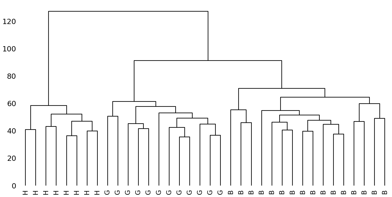
The tree should be read from bottom to top, where the original texts are displayed as the tree’s leaf nodes. When moving to the top, we see how these original nodes are progressively being merged in new nodes by vertical branches. Subsequently, these newly created, non-original nodes are eventually joined into higher-level nodes and this process continues until all nodes have been merged into a single root node at the top. On the vertical axis, we see numbers which we can read as the distance between the various nodes: the longer the branches that lead up to a node, the more distant the nodes that are being merged. The cluster analysis performs well: the tree splits into three coherent clusters, each consisting solely of texts from one author.

How do the documents with unknown authorship fit into this tree? After “stacking” their document vectors to those of the entire corpus, we rerun the cluster analysis, which produces the tree below.

Note

The reader should note that we use the function transform() on the vectorizer and scaler, rather than fit() or fit_transform(), because we do not wish to re-fit these and use them in the exact same way as they were applied to the texts of undisputed authorship.

v_test_docs = vectorizer.transform(test_docs[1:])
v_test_docs = preprocessing.normalize(v_test_docs.astype(float), norm='l1')
v_test_docs = scaler.transform(v_test_docs.toarray())

all_documents = np.vstack((v_documents, v_test_docs))

dm = scidist.pdist(all_documents, 'cityblock')
linkage_object = hierarchy.linkage(dm, method='complete')

plot_tree(linkage_object, authors + test_titles[1:], figsize=(12, 5))

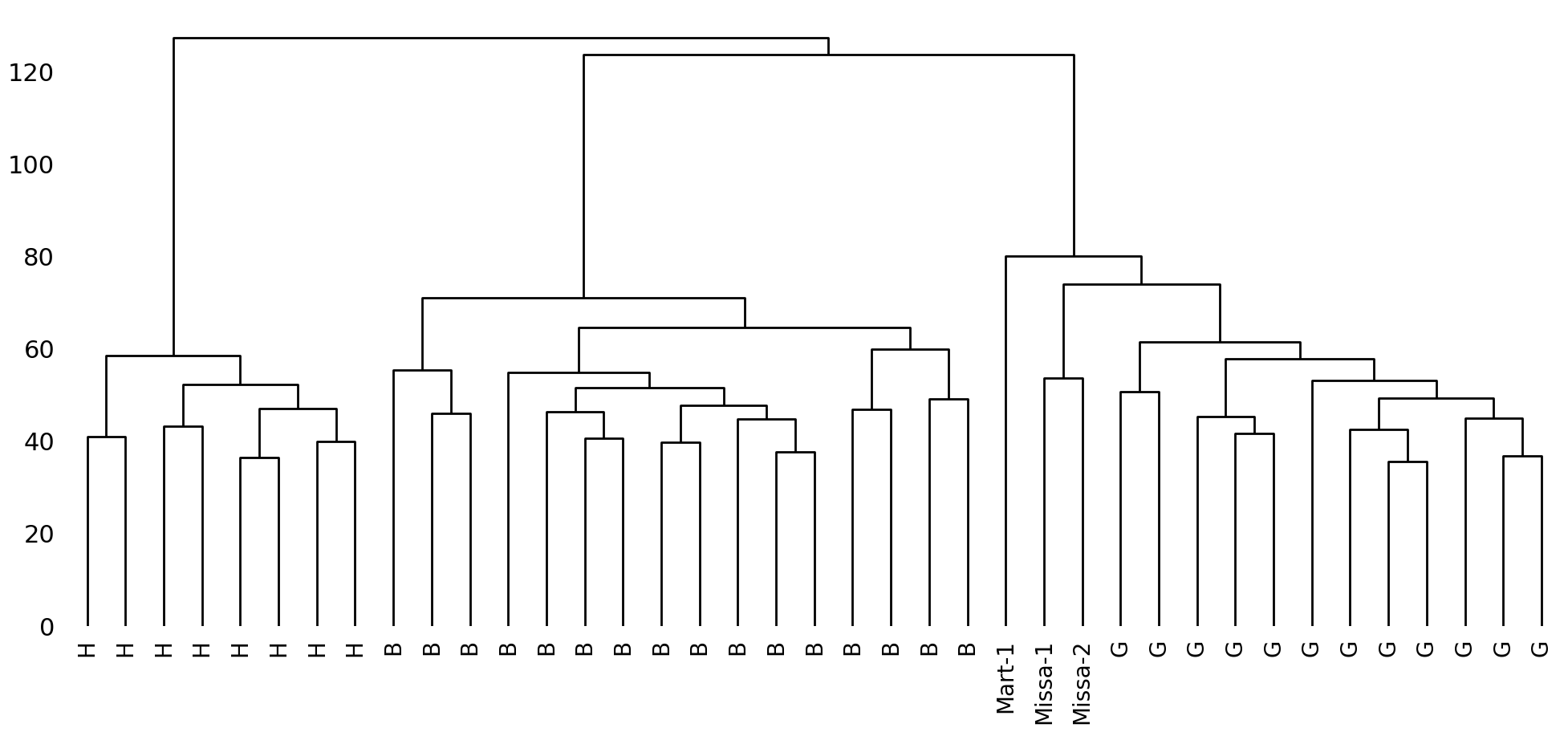
Interestingly, and even without normalizing the document length (to unclutter the visualization), the disputed texts are clustered together with documents written by Guibert of Gembloux. The relatively high branching position of D_Mart.txt suggests that it is not at the core of his writings, but the similarities are still striking. The cluster analysis thus adds some nuance to our prior results, and provides new hypotheses worth exploring. In the next section, we will explore a second “clustering” technique to add yet another perspective to the mix.

Principal Component Analysis#

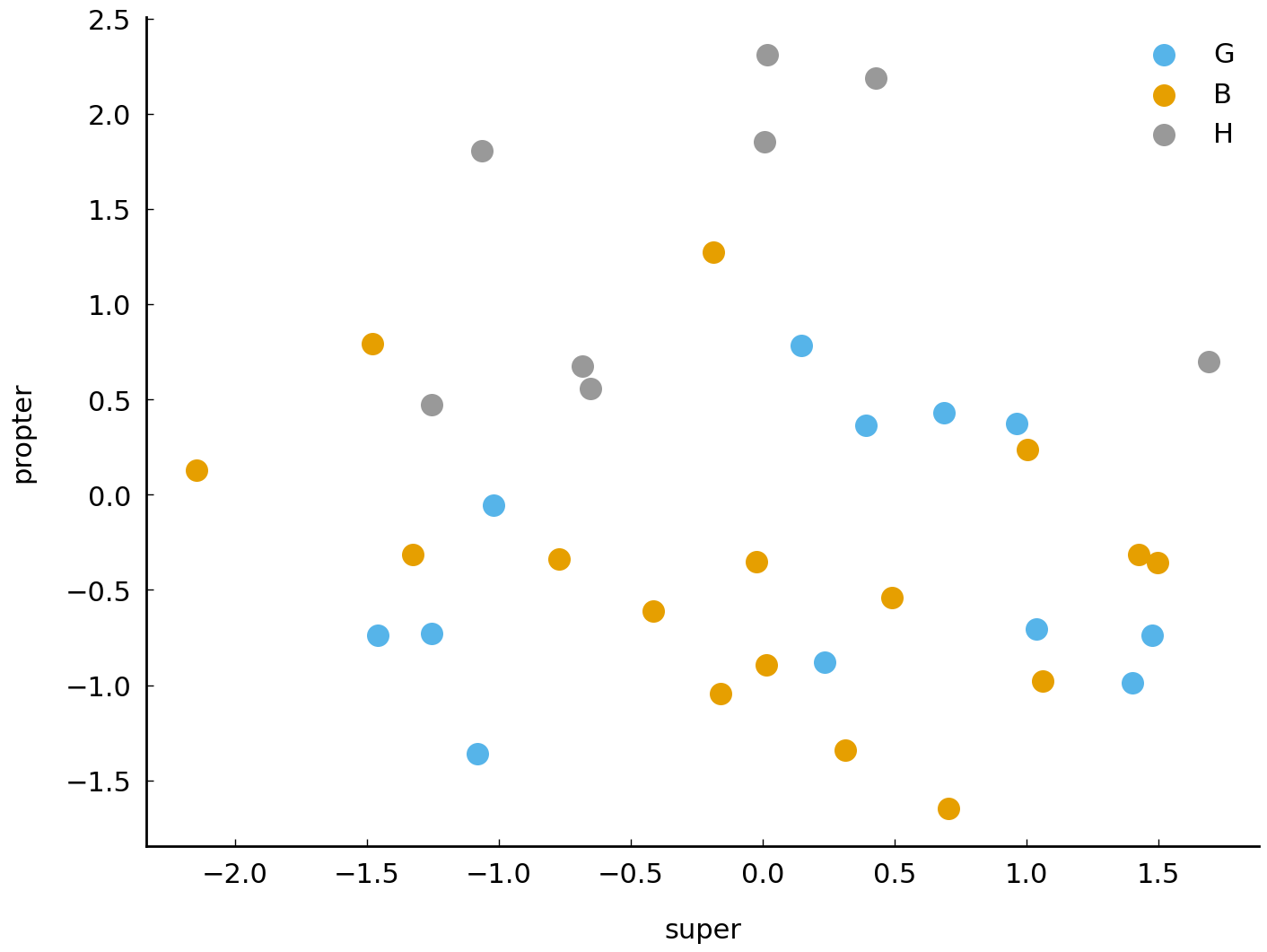
In this final section, we will a cover a common technique in stylometry, called Principal Component Analysis (or PCA). PCA stems from multivariate statistics, and has been applied regularly to literary corpora in recent years [Binongo and Smith, 1999, Hoover, 2007]. PCA is a useful technique for textual analysis because it enables intuitive visualizations of corpora. The document-term matrix created earlier represents a \(36 \times 65\) matrix: i.e., we have 36 documents (by 3 authors) which are each characterized in terms of 65 word frequencies. The columns in such a matrix are also called dimensions, because our texts can be considered points in a geometric space that has 65 axes. We are used to plotting such points in a geometric space that only has a small number of axes (e.g., 2 or 3), using the pairwise coordinates, reflecting their score in each dimension. Let us plot, for instance, these texts with respect to two randomly selected dimensions (i.e., those representing super and propter):

words = list(vectorizer.get_feature_names_out())
authors = np.array(authors)
x = v_documents[:, words.index('super')]
y = v_documents[:, words.index('propter')]

fig, ax = plt.subplots()
for author in set(authors):
    ax.scatter(x[authors==author], y[authors==author], label=author)
ax.set(xlabel='super', ylabel='propter')
plt.legend();

To make our plot slightly more readable, we could plot the author’s name for each text, instead of multi-colored dots. For this, we first need to plot an empty scatter plot, with invisible points using scatter(). Next, we overlay these points in their vertical and horizontal center with a string label. The resulting plot is shown below:

fig, ax = plt.subplots()
ax.scatter(x, y, facecolors='none')
for p1, p2, author in zip(x, y, authors):
    ax.text(p1, p2, author[0], fontsize=12,
            ha='center', va='center')
ax.set(xlabel='super', ylabel='propter');

findfont: Font family ['sans-serif'] not found. Falling back to DejaVu Sans.

findfont: Generic family 'sans-serif' not found because none of the following families were found: "Roboto Condensed Regular"

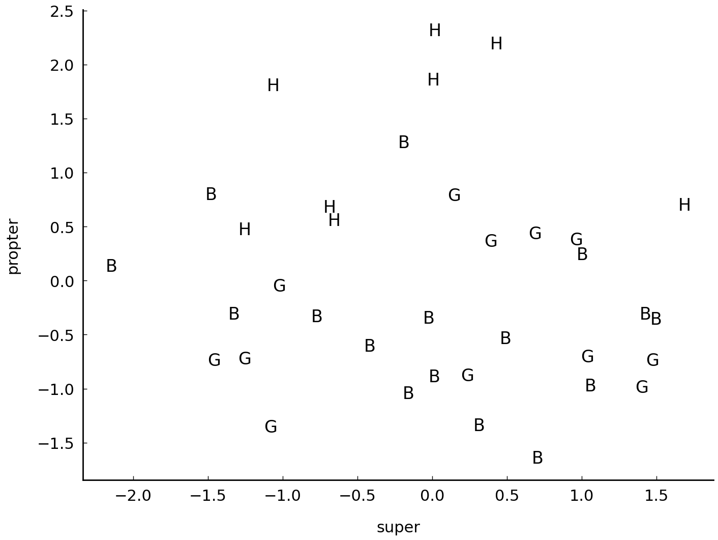
The sad reality remains that we are only inspecting 2 of the 65 variables that we have for each data point. Humans have great difficulties imagining, let alone plotting, data in more than 3 dimensions simultaneously. Many real-life datasets even have much more than 65 dimensions, so that the problem becomes even more acute in those cases. PCA is one of the many techniques which exist to reduce the dimensionality of datasets. The general idea behind dimensionality reduction is that we seek a new representation of a dataset, which needs much less dimensions to characterize our data points, but which still offers a maximally faithful approximation of our data. PCA is prototypical approach to text modeling in stylometry, because we create a much smaller model which we know beforehand will only be an approximation of our original dataset. This operation is often crucial for scholars who deal with large datasets, where the number of features is much larger that the number of data points. In stylometry, it is very common to reduce the dimensionality of a dataset to as little as 2 or 3 dimensions.

Applying PCA#

Before going into the intuition behind this technique, it makes sense to get a rough idea of the kind of output which a PCA can produce. Nowadays, there are many Python libraries which allow you to quickly run a PCA. The aforementioned scikit-learn library has a very efficient, uncluttered object for this. Below, we instantiate such an object and use it to reduce the dimensionality of our original \(36 \times 65\) matrix:

import sklearn.decomposition

pca = sklearn.decomposition.PCA(n_components=2)
documents_proj = pca.fit_transform(v_documents)

print(v_documents.shape)
print(documents_proj.shape)

(36, 65)
(36, 2)

Note that the shape information shows that the dimensionality of our new dataset is indeed restricted to n_components, the parameter which we set at 2 when calling the PCA constructor. Each of these newly created columns is called a “principal component” (PC), and can be expected to describe an important aspect about our data. Apparently, the PCA has managed to provide a two-dimensional “summary” of our data set, which originally contained 65 columns. Because our dataset is now low-dimensional, we can plot it using the same plotting techniques that were introduced above.

c1, c2 = documents_proj[:, 0], documents_proj[:, 1]

fig, ax = plt.subplots()
ax.scatter(c1, c2, facecolors='none')

for p1, p2, author in zip(c1, c2, authors):
    ax.text(p1, p2, author[0], fontsize=12,
            ha='center', va='center')

ax.set(xlabel='PC1', ylabel='PC2');

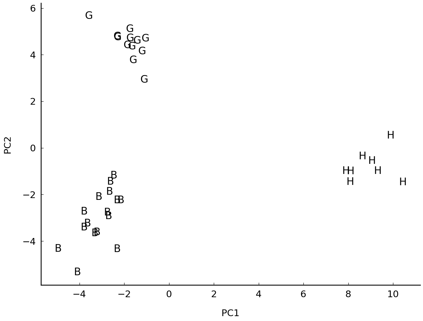
By convention, we plot the first component on the horizontal axis and the second component on the vertical axis. The resulting plot displays much more authorial structure: the texts now form very neat per-author clusters. Like hierarchical clustering, PCA too is an unsupervised method: we never included any provenance information about the texts in the analysis. Therefore it is fascinating that the analysis still seems to be able to automatically distinguish between the writing styles of our three authors. The first component is responsible for the horizontal distribution of our texts in the plot; interestingly, we see that this component primarily manages to separate Hildegard from her two male contemporaries. The second component, on the other hand, is more useful to distinguish Bernard of Clairvaux from Guibert of Gembloux on the vertical axis. This is also clear from the more simplistic visualization shown below, which was generated by the following lines of code:

fig, ax = plt.subplots()

for idx in range(pca.components_.shape[0]):
    ax.axvline(idx, linewidth=2, color='lightgrey')
    for score, author in zip(documents_proj[:, idx], authors):
        ax.text(
            idx, score, author[0], fontsize=10,
            va='center', ha='center')

ax.axhline(0, ls='dotted', c='black')
ax.set(
    xlim=(-0.5, 1.5), ylim=(-12, 12),
    xlabel='PCs', ylabel='Component scores',
    xticks=[0, 1], xticklabels=["PC1", "PC2"]);

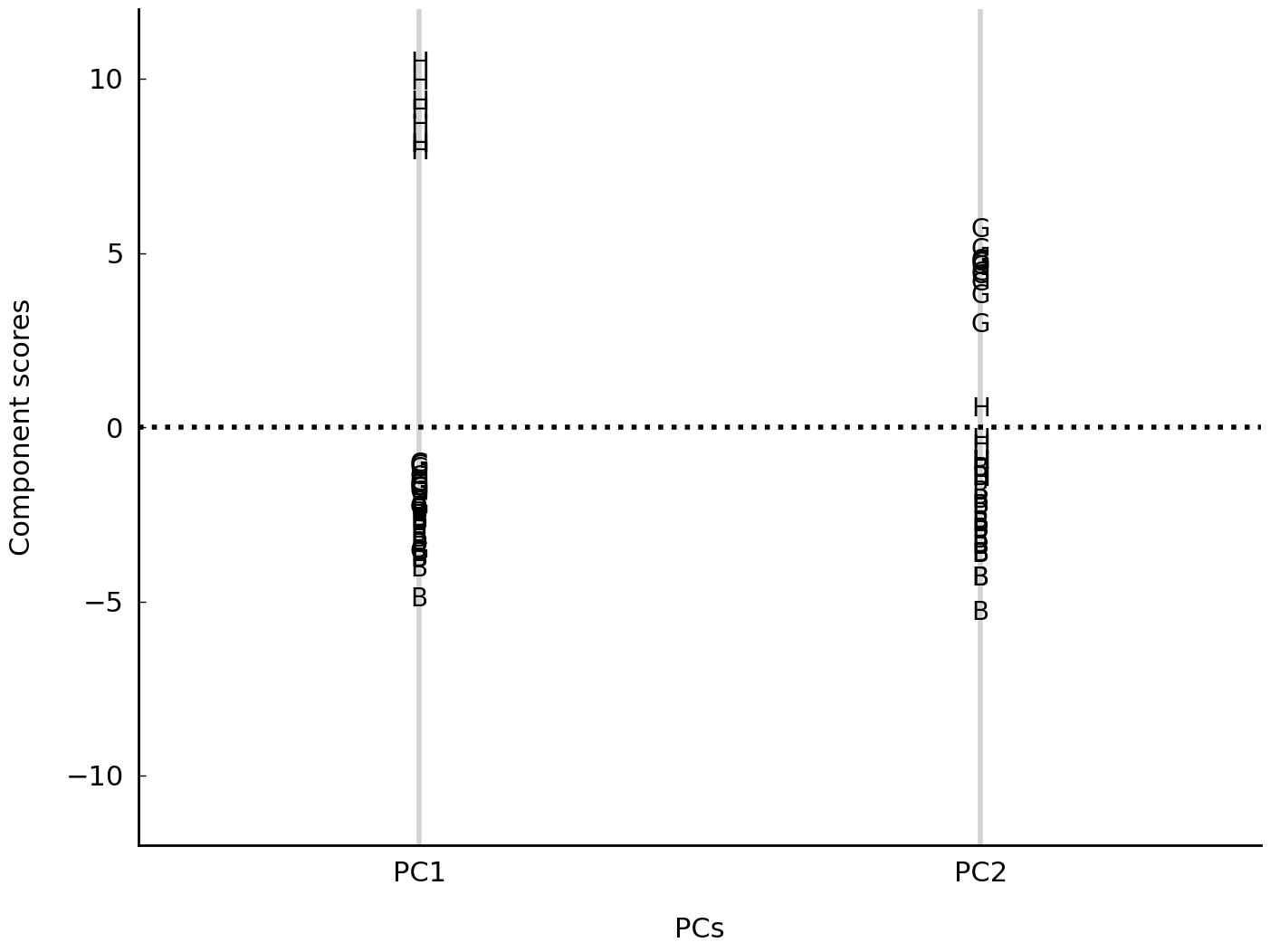
Note how the distribution of samples in the first component realizes a clear distinction between Hildegard and the rest. The clear distinction collapses in the second component, but, interestingly, this second component shows a much clearer opposition between the two other authors.

The intuition behind PCA#

How does PCA work? A formal description of PCA requires some familarity with linear algebra (see, for example, Shlens [2014]). When analyzing texts in terms of word frequencies, it is important to realize that there exist many subtle correlations between such frequencies. Consider the pair of English articles the and a: whenever a text shows an elevated frequency of the definite article, this increases the likelihood that the indefinite article will be less frequent in that same text. That is because the and a can be considered “positional synonyms”: these articles can never appear in the same syntactic slot in a text (they exclude each other), so that authors, when creating noun phrases, must choose between one of them. This automatically entails that if an author has a clear preference for indefinite articles, (s)he will almost certainly use less definite articles. Such a correlation between two variables could in fact also be described by a single new variable \(y\). If a text has a high score for this abstract variable \(y\), this could mean that (s)he uses a lot of definite articles but much less indefinite articles. A low, negative score for \(y\) might on the other hand represent the opposite situation, where an author clearly favors indefinite over definite articles. Finally, a \(y\)-score of zero could mean that an author does not have a clear preference. This abstract \(y\)-variable is a simple example but it can be likened to a principal component. A PCA too will attempt to compress the information contained in word frequencies, by coming up with new, compressed components that decorrelate this information and summarize it into a far smaller number of dimensions. Therefore, PCA will often indirectly detect subtle oppositions between texts that are interesting in the context of authorship attribution. Let us take back a number of steps:

pca = sklearn.decomposition.PCA(n_components=2)
pca.fit(v_documents)

print(pca.components_.shape)

(2, 65)

We get back a matrix of which the shape (\(2 \times 65\)) will look familiar: we have two principal components (cf. n_components) that each have a score for the original word features in the original document-term matrix. Another interesting property of the pca object is the explained variance ratio:

pca = sklearn.decomposition.PCA(n_components=36)
pca.fit(v_documents)

print(len(pca.explained_variance_ratio_))

The explained_variance_ratio_ attribute has a score for each of the 36 principal components in our case. These are normalized scores and will sum to 1:

print(sum(pca.explained_variance_ratio_))

1.0

Intuitively, the explained variance expresses for each PC how much of the original variance in our dataset it retains, or, in other words, how accurately it offers a summary of the original data when considered in isolation. Components are typically ranked according to this criterium, so that the first principal component (cf. the horizontal dimension above) is the PC which, in isolation, preserves most of the original variation in the original data. Typically, only 2 or 3 components are retained, because when taken together, one will often see that these PCs already explain the bulk of the original variance, so that the rest can be safely dropped. Also, components that have an explained variance < 0.05 are typically ignored because they add very little information in the end [Baayen, 2008]. We can visualize this distribution using a small bar plot, where the bars indicate the explained variance for and in which we also keep track of the cumulative variance that is explained as we work our way down the component list.

var_exp = pca.explained_variance_ratio_
cum_var_exp = np.cumsum(var_exp)

fig, ax = plt.subplots()

ax.bar(range(36), var_exp, alpha=0.5, align='center',
        label='individual explained variance')

ax.step(range(36), cum_var_exp, where='mid',
         label='cumulative explained variance')

ax.axhline(0.05, ls='dotted', color="black")
ax.set(ylabel='Explained variance ratio', xlabel='Principal components')
ax.legend(loc='best');

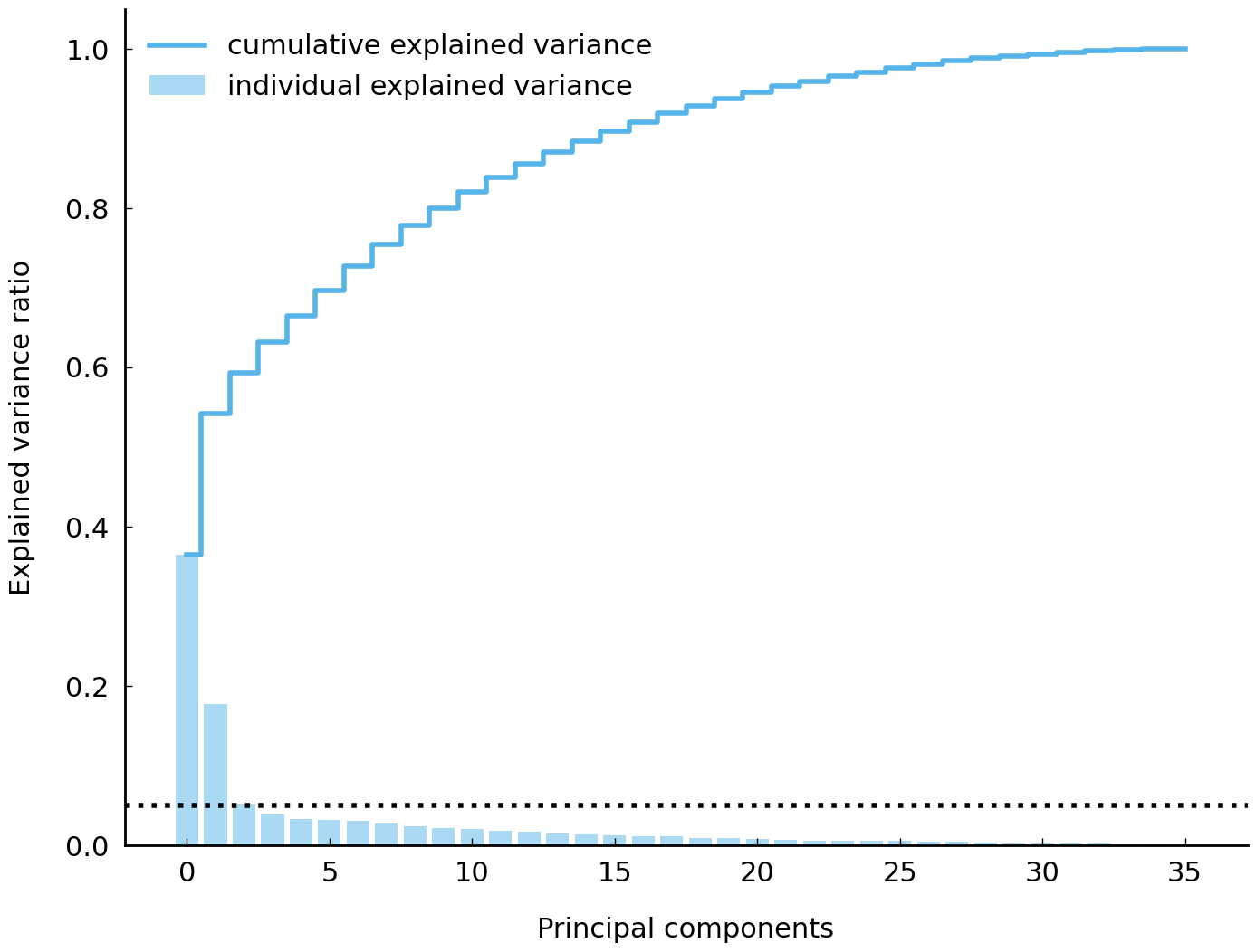
As you can see, the first three components together explain a large proportion of the original variance; the subsequent PCs add relatively little, with only the first few PCs reaching the 0.05 level (which is plotted as a dotted black line). Surprisingly, we see that the first component alone can account for a very large share of the total variance. In terms of modeling, the explained variance score is highly valuable: when you plot texts in their first two components as we did, it is safe to state that the total variance explained amounts to the following plain sum:

print(var_exp[0] + var_exp[1])

0.5418467851530999

Thus, the PCA does not only yield a visualization, but it also yields a score expressing how faithful this representation is with respect to the original data. This score is on the one hand relatively high, given the fact that we have reduced our complete dataset to a compressed format of just two columns. On the other hand, we have to remain aware that the other components might still capture relevant information about our texts that a two-dimensional visualization does not show.

Loadings#

What do the components, yielded by a PCA, look like? Recall that, in scikit-learn, we can easily inspect these components after a PCA object has been fitted:

pca = sklearn.decomposition.PCA(n_components=2).fit(v_documents)
print(pca.components_)

[[-0.01261718 -0.17502663  0.19371289 ... -0.05284575  0.15797111
  -0.14855212]
 [ 0.25962781  0.0071369   0.05184334 ... -0.05141676 -0.06927065
   0.04312771]]

In fact, applying the fitted pca object to new data (i.e., the transform() step), comes down to a fairly straightforward multiplication of the original data matrix with the component matrix. The only step which scikit-learn adds is the subtraction of the columnwise mean in the original matrix, to center values around a mean of zeros. (Don’t mind the transpose() method for now, we will explain it shortly.)

X_centered = v_documents - np.mean(v_documents, axis=0)
X_bar1 = np.dot(X_centered, pca.components_.transpose())
X_bar2 = pca.transform(v_documents)

The result is, as you might have expected, a matrix of shape \(36 \times 2\), i.e., the coordinate pairs which we already used above. The numpy.dot() function which we use in this code block refers to a so-called dot product, which is a specific type of matrix multiplication (cf. chapter Exploring Texts using the Vector Space Model). Such a matrix multiplication is also called a linear transformation, where each new component will assign a specific weight to each of the original feature scores. These weights, i.e., the numbers contained in the components matrix, are often also called loadings, because they reflect how important each word is to each PC. A great advantage of PCA is that it allows us to inspect and visualize these weights or loadings in a very intuitive way, which allows us to interpret the visualization in an even more concrete way: we can plot the word loadings in a scatter plot too, since we can align the component scores with the original words in our vectorizer’s vocabulary. For our own convenience, we first transpose the component matrix, meaning that we flip the matrix and turn the row vectors into column vectors.

print(pca.components_.shape)
comps = pca.components_.transpose()
print(comps.shape)

(2, 65)
(65, 2)

This is also why we needed the transpose() method a couple of code blocks ago, since we needed to make sure that dimensions of both X and the components matrix matched. We can now more easily “zip” this transposed matrix with our vectorizer’s vocabulary, and sort these words according to their loadings on PC1:

import operator

vocab = vectorizer.get_feature_names_out()
vocab_weights = sorted(zip(vocab, comps[:, 0]), key=operator.itemgetter(1), reverse=True)

We can now inspect the top and bottom of this ranked list to find out which items have the strongest loading (either positive or negative) on PC1:

print('Positive loadings:')
print('\n'.join(f'{w} -> {s}' for w, s in vocab_weights[:5]))

Positive loadings:
in -> 0.19371288677377668
ita -> 0.18241992378624636
per -> 0.18115806688500907
uelut -> 0.1801888293185639
unde -> 0.1762194975035874

print('Negative loadings:')
print('\n'.join(f'{w} -> {s}' for w, s in vocab_weights[-5:]))

Negative loadings:
quam -> -0.16396980041076892
iam -> -0.16589861024232344
magis -> -0.16743388326578998
aut -> -0.17037738587759382
qui -> -0.17502663330844656

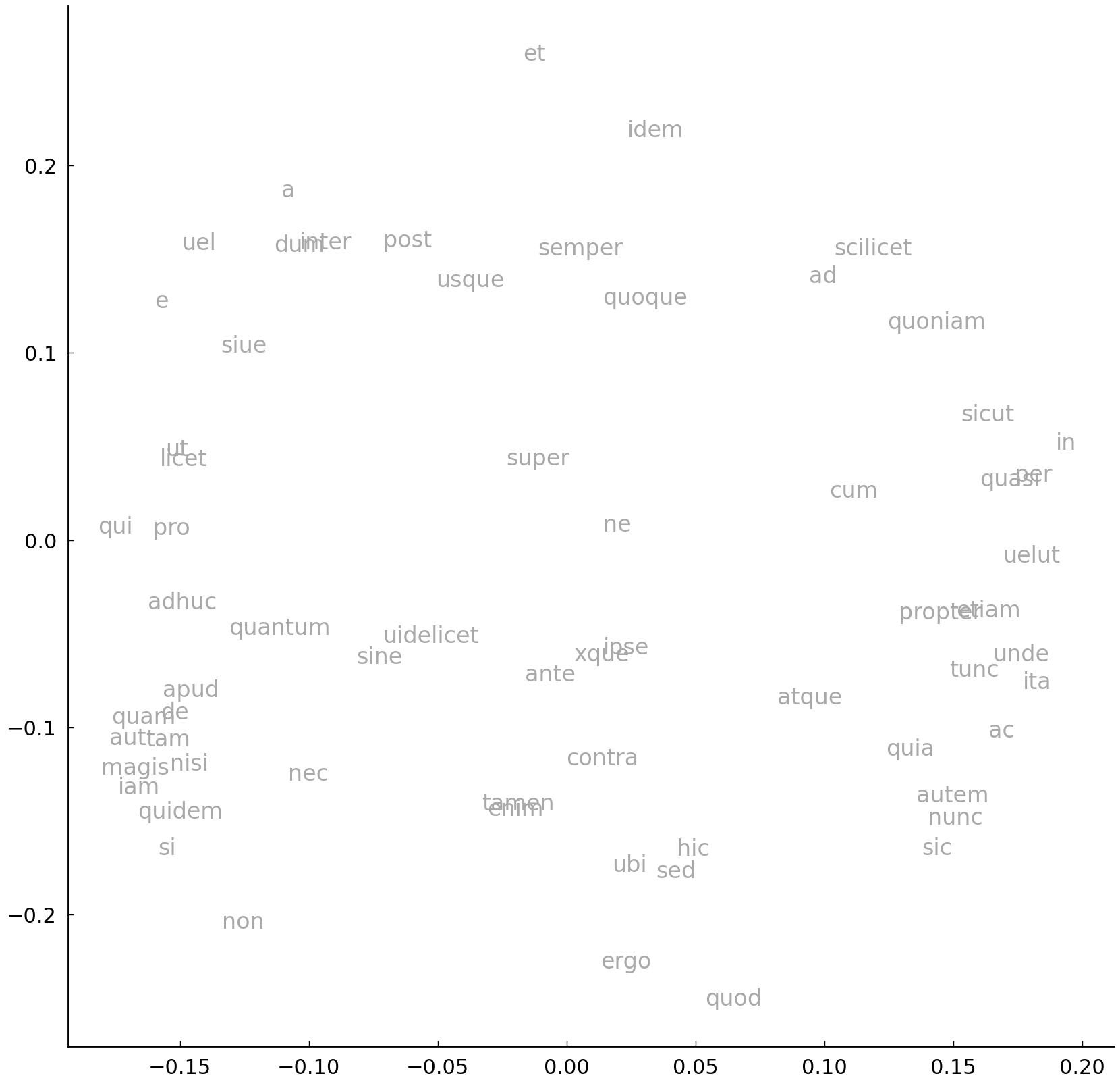
Now that we understand how each word has a specific “weight” or importance for each component, it becomes clear that, instead of the texts, we should also be able to plot the words in the two-dimensional space, defined by the component matrix. The visualization is shown below; the underlying code runs entirely parallel to our previous scatter plot code:

l1, l2 = comps[:, 0], comps[:, 1]

fig, ax = plt.subplots(figsize=(10, 10))
ax.scatter(l1, l2, facecolors='none')

for x, y, l in zip(l1, l2, vocab):
    ax.text(x, y, l, ha='center', va='center', color='darkgrey', fontsize=12)

It becomes truly interesting if we first plot our texts, and then overlay this plot with the loadings plot. We can do this by plotting the loadings on the so-called twin axis, opposite of the axes on which we first plot our texts. A full example, which adds additional information, reads as follows.

import mpl_axes_aligner.align

def plot_pca(document_proj, loadings, var_exp, labels):
    # first the texts:
    fig, text_ax = plt.subplots(figsize=(10, 10))
    x1, x2 = documents_proj[:, 0], documents_proj[:, 1]
    text_ax.scatter(x1, x2, facecolors='none')
    for p1, p2, author in zip(x1, x2, labels):
        color = 'red' if author not in ('H', 'G', 'B') else 'black'
        text_ax.text(p1, p2, author, ha='center',
                     color=color, va='center', fontsize=12)

    # add variance information to the axis labels:
    text_ax.set_xlabel(f'PC1 ({var_exp[0] * 100:.2f}%)')
    text_ax.set_ylabel(f'PC2 ({var_exp[1] * 100:.2f}%)')

    # now the loadings:
    loadings_ax = text_ax.twinx().twiny()
    l1, l2 = loadings[:, 0], loadings[:, 1]
    loadings_ax.scatter(l1, l2, facecolors='none');
    for x, y, loading in zip(l1, l2, vectorizer.get_feature_names_out()):
        loadings_ax.text(x, y, loading, ha='center', va='center',
                         color='darkgrey', fontsize=12)

    mpl_axes_aligner.align.yaxes(text_ax, 0, loadings_ax, 0)
    mpl_axes_aligner.align.xaxes(text_ax, 0, loadings_ax, 0)
    # add lines through origins:
    plt.axvline(0, ls='dashed', c='lightgrey', zorder=0)
    plt.axhline(0, ls='dashed', c='lightgrey', zorder=0);

# fit the pca:
pca = sklearn.decomposition.PCA(n_components=2)
documents_proj = pca.fit_transform(v_documents)
loadings = pca.components_.transpose()
var_exp = pca.explained_variance_ratio_

plot_pca(documents_proj, loadings, var_exp, authors)

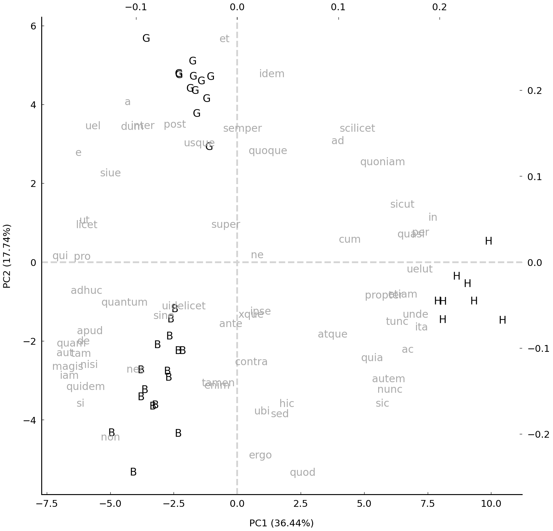
Such plots are great visualizations because they show the main stylistic structure in a dataset, together with an indication of how reliable each component is. Additionally, the loadings make clear which words have played an important role in determining the relationships between texts. Loadings which can be found to the far left of the plot can be said to be typical of the texts plotted in the same area. As you can see in this analysis, there are a number of very common lemmas which are used in rather different ways by the three authors: Hildegard is a frequent user of in (probably because she always describes things she witnessed in visions), while the elevated use of et reveals the use of long, paratactic sentences in Guibert’s prose. Bernard of Clairvaux uses non rather often, probably as a result of his love for antithetical reasonings. Metaphorically, the loadings can be interpreted as little “magnets”: when creating the scatter plot, you can imagine that the loadings are plotted first. Next, the texts are dropped in the middle of the plot and then, according to their word frequencies, they are attracted by the word magnets, which will eventually determine their position in the diagram.

Therefore, loading plots are a great tool for the interpretation of the results of a PCA. A cluster tree acts much more like a black box in this respect, but these dendrograms can be used to visualize larger datasets. In theory, a PCA visualization that is restricted to just two or three dimensions is not meant to visualize large datasets that include more than ca. three to four oeuvres, because two dimensions can only visualize so much information [Binongo and Smith, 1999]. One final advantage, from a theoretical perspective, is that PCA explicitly tries to model the correlations which we know exist between word variables. Distance metrics, such as the Manhattan distance used in Delta or cluster analyses, are much more naïve in this respect, because they do not explicitly model such subtle correlations.

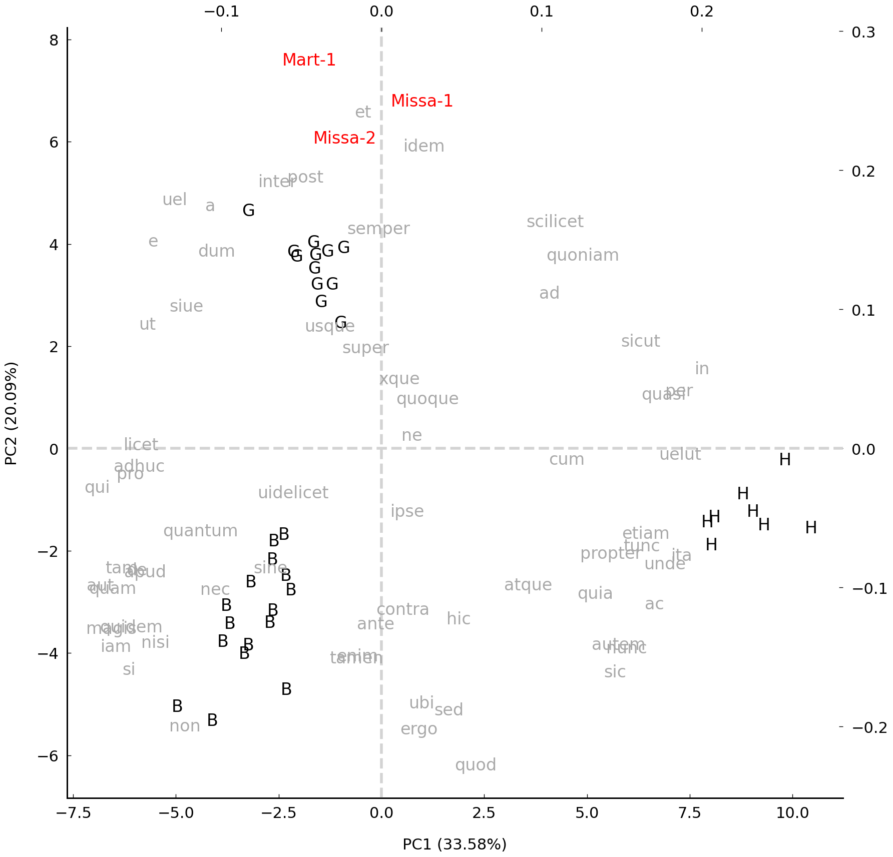
We are now ready to include the other texts of disputed authorship in this analysis—these are displayed in red in the figure below, but we exclude the previously analyzed test text by Bernard of Clairvaux. We have arrived at a stage in our analysis where the result should look reasonably similar to the graph which was shown in the beginning of the chapter, because we followed the original implementation as closely as possible. The texts of doubtful provenance are clearly drawn to the area of the space which is dominated by Guibert’s samples (indicated with the prefix G_): the scatter plot therefore reveals that the disputed documents are much more similar, in term of function word frequencies, to the oeuvre of Guibert of Gembloux, Hildegard’s last secretary, than to works of the mystic herself. The very least we can conclude from this analysis is that these writing samples cannot be considered typical of Hildegard’s writing style, which should fuel doubts about their authenticity, in combination with other historic evidence.

all_documents = preprocessing.scale(np.vstack((v_documents, v_test_docs)))
pca = sklearn.decomposition.PCA(n_components=2)
documents_proj = pca.fit_transform(all_documents)
loadings = pca.components_.transpose()
var_exp = pca.explained_variance_ratio_

plot_pca(documents_proj, loadings, var_exp, list(authors) + test_titles[1:])

Conclusions#

Authorship is an old and important problem in philology but, nowadays, stylistic authentication problems are studied in a much more diverse set of fields, including forensic linguistics and internet safety studies. Computational modeling brings added value to many societally relevant problems as such and is often less biased than human readers in performing this difficult task. Any serious authentication study in the humanities, however, should not rely on hard numbers alone: additional, text-external evidence must always be carefully taken into account and whenever one encounters an attribution result that diametrically opposes results obtained by conventional studies, that should be a cause for worry.

At the same time, stylometry often brings fresh quantitative evidence to the table that might call into question preconveived ideas about the authorship of texts. The case study presented above, for instance, raised interesting questions about a text, of which the authorship for centuries went undisputed. At the same, the reader should note that the Hildegard scholars involved in this research (Jeroen Deploige and Sarah Moens) still chose to edit the disputed texts as part of Hildegard opera omnia, because the ties to her oeuvre were unmistakable. This should remind us that authorship and authenticity are often more a matter of (probabilistic) degree than of a (boolean) kind. Exactly because of these scholarly gradients, quantitative approaches are useful to help objectify our own intuitions.

Exercises#

Easy#

Julius Caesar (100–44 BC), the famous Roman statesman, was also an accomplished writer of Latin prose. He is famous for his collection of war commentaries, including the Bellum Civile, offering an account of the civil war, and the Bellum Gallicum, where he reports on his military expeditions in Gaul. Caesar wrote the bulk of these texts himself, with the exception of book eight of the Gallic Wars, which is believed to have been written by one of Caesar’s generals, Aulus Hirtius. Three other war commentaries survive in the Caesarian tradition, which have sometimes been attributed to Caesar himself: the Alexandrian War (Bellum Alexandrinum), the African War (Bellum Africum), and the Spanish War (Bellum Hispaniense). It remains unclear, however, who actually authored these: Caesar’s ancient biographer Suetonius, for instance, suggests that either Hirtius or another general, named Oppius, authored the remaining works.

Kestemont et al. [2016] argue using stylometric arguments that, in all likelihood, Hirtius indeed authored one of these other works, whereas the other two commentaries were probably not written by either Caesar or Hirtius. Although this publication used a fairly complex authorship verification technique, a plain cluster analysis, like the one introduced in the previous section, can also be used to set up a similar argument. This is what we will do in the following set of exercises.

The dataset is stored as a compressed tar archive, caesar.tar.gz, which can be decompressed using the following lines of code:

import tarfile

tf = tarfile.open('data/caesar.tar.gz', 'r')
tf.extractall('data')

After decompressing the archive, you can find a series of texts under data/caesar, which represent consecutive 1000-word segments which we extracted from these works. The plain text file caesar_civ3_6.txt, for instance, represents the sixth 1000-word sample from the third book of the civil war commentary by Caesar, whereas Hirtius’s contributions to book 8 of the Gallic Wars take the prefix hirtius_gall8. Samples containing the codes alex, afric, and hispa contain samples of the dubious war commentaries.

Load the texts from disk, and store them in a list (texts). Keep a descriptive label for each text (e.g., gall8) in a parallel list (titles) and fill yet another list (authors) with the author labels. How many texts are there in the corpus?
Convert the texts into a vector space model using the CountVectorizer object, and keep only the 10,000 most frequent words. Print the shape of the vector space model, and confirm that the number of rows and columns is correct.
Normalize the counts into relative frequencies (i.e., apply \(L1\) normalization).

Moderate#

Use the normalized frequencies to compute the pairwise distances between all documents in the corpus. Choose an appropriate distance metric, and motivate your choice.
Run a hierarchical agglomerative cluster analysis on the computed distance matrix. Plot the results as a dendrogram using the function plot_tree(). Which of the dubious texts is generally closest in style to Hirtius’s book 8?
Experiment with some other distance metrics and recompute the dendrogram. How does the choice for a particular distance metric impact the results?

Challenging#

Jack the Ripper is one of the most famous and notorious serial killers of the nineteenth century. Perhaps fueled by the fact that he was never apprehended or identified, the mystery surrounding the murders in London’s Whitechapel district has only grown with time. Around the time of the murders (and also in the following years), Jack allegedly sent numerous letters to the police announcing and / or describing his crimes, which shrouded the crimes in even deeper mystery. However, there are several reasons why the authenticity of most of these letters has always remained contentious.

In a recent study, Nini [2018] sheds new light on the legitimacy of these letters using stylometric methods. Nini explains that the legitimacy is doubtful since a significant number of letters have been sent from different places all around the United Kingdom, which, although not strictly impossible, makes it unlikely that they have the same sender. As explained by Nini [2018], this adds to the suspicion that many of these are hoax letters, maybe even written by journalists, in an attempt to increase newspaper sales.

Nini’s study focuses in particular on four early letters that were received not later than October 1, 1888, by the London police: crucially, these letters antedate the wider publication among the general public of the contents of the earliest letters. The four “prepublication” letters are marked in the dataset through the presence of the following shorthand codes: SAUCY JACKY, MIDIAN, DEAR BOSS, FROM HELL. If these documents were authored by the same individual, this would constitute critical historical evidence, or, as Nini notes: “these four texts are particularly important because any linguistic similarity that links them cannot be explained by influence from the media, an explanation that cannot be ruled out for the other texts”.

In the following exercises, we will try to replicate some of his findings, and assess whether the “prepublication” letters were written by the same person.

The Jack the Ripper corpus used in Nini [2018] is saved as a compressed tar archive under data/jack-the-ripper.tar.gz. Load the text files in a list, and convert the filenames into a list of clearly readable labels (i.e., take the actual filename and remove the extension). Construct a vector space model of the texts using scikit-learn’s CountVectorizer. From the original paper [Nini, 2018], a number of crucial preprocessing details are available that allow you to approximate the author’s approach when instantiating the CountVectorizer. Consult the online documentation:
- The paper relies on word bigrams as features (i.e., sequences of two consecutive words), rather than individual words or word “unigrams”, as we have done before (cf. ngram_range parameter).
- Since all texts are relatively short, Nini refrains from using actual frequencies (as these would likely be unreliable), and uses binary features instead (cf. binary parameter).
- The author justifies at length why he chose to remove a small set of eight very common bigrams that occur in more than 20% of all documents in the corpus (cf. max_df parameter).
- The author explicitly allows one-letter words into the vocabulary (e.g. I or a), so make sure to reuse the token_pattern regex used above and not the default setting. Finally, use sklearn.preprocessing.scale() to normalize the values in the resulting matrix in a column-wise fashion (axis=1).
Perform a hierarchical cluster analysis on the corpus using the Cosine Distance metric and Ward linkage (as detailed in the paper). The resulting tree will be hard to read, because it has many more leaf nodes than the examples in the chapter. First, read through the documentation of the dendrogram() function in scipy.cluster.hierarchy. Next, customize the existing plot_tree() function to improve the plot’s readability:
- Change the “orientation” argument to obtain a vertical tree (i.e., with the leaf nodes on the Y axis). In this new setup, you might also want to adapt the leaf_rotation argument.
- Find a way to color the nodes of the prepublication letters. This is not trivial, since you will need to access the labels in the plot (after drawing it) but you also need to extract some information from the dictionary returned by the dendrogram() function.
- Provide a generous figsize to make the resulting graph maximally readable (e.g., (10, 40)).
Do the results confirm Nini [2018]’s conclusions that some of the “prepublication letters” could very well be written by the same author? Which ones (not)?
A PCA as described in this chapter can help to gain more insight into the features underlying the distances between the texts. Run a PC analysis on the corpus, and plot your results using the plot_pca() function defined above. At first, however, the scatter plot will be very hard to read. Implement the following customizations to the existing code:
- Color the prepublication letters in red.
- Because the vocabulary is much larger than above, we need to unclutter the visualization. Restrict the number of loadings that you pass to plot_pca(), by selecting the loadings with the most extreme values for the first two components. One way of doing this is to multiply both component scores for each word with one another and then take the absolute value. If the resulting scores are properly ranked, the highest values will reveal the most extreme, and therefore most interesting, loadings.
Nini argues that one of the four prepublications is of a different authorial provenance than the other three. Can you single out particular bigrams that are typical of this letter and untypical of the others?

Humanities Data Analysis: Case Studies with Python

Stylometry and the Voice of Hildegard

Contents