Introduction
Contents
Introduction#
Quantitative Data Analysis and the Humanities#
The use of quantitative methods in humanities disciplines such as history, literary studies, and musicology has increased considerably in recent years. Now it is not uncommon to learn of a historian using geospatial data, a literary scholar applying techniques from computational linguistics, or a musicologist employing pattern matching methods. Similar developments occur in humanities-adjacent disciplines, such as archeology, anthropology, and journalism. An important driver of this development, we suspect, is the advent of cheap computational resources as well as the mass digitization of libraries and archives [Abello et al., 2012, Borgman, 2010, Imai, 2018, Van Kranenburg et al., 2017] It has become much more common in humanities research to analyze thousands, if not millions, of documents, objects, or images; an important part of the reason why quantitative methods are attractive now is that they promise the means to detect and analyze patterns in these large collections.
A recent example illustrating the promise of data-rich book history and cultural analysis is Bode [2012]. Bode’s analysis of the massive online bibliography of Australian literature AusLit demonstrates how quantitative methods can be used to enhance our understanding of literary history in ways that would not be possible absent data-rich and computer-enabled approaches. Anchored in the cultural materialist focus of Australian literary studies, Bode uses data analysis to reveal unacknowledged shifts in the demographics of Australian novelists, track the entry of British publishers into the Australian book market in the 1890s, and identify ways Australian literary culture departed systematically from British practices. A second enticing example showing the potential of data-intensive research is found in Da Silva and Tehrani [2016]. Using data from large-scale folklore databases, Da Silva and Tehrani [2016] investigate the international spread of folktales. Based on quantitative analyses, they show how the diffusion of folktales is shaped by language, population histories, and migration. A third and final example—one that can be considered a landmark in the computational analysis of literary texts—is the influential monograph by Burrows [1987] on Jane Austen’s oeuvre. Burrows uses relatively simple statistics to analyze the frequencies of inconspicuous, common words that typically escape the eye of the human reader. In doing so he documents hallmarks of Austen’s sentence style and carefully documents differences in characters’ speaking styles. The book illustrates how quantitative analyses can yield valuable and lasting insights into literary texts, even if they are not applied to datasets that contain millions of texts.
Although recent interest in quantitative analysis may give the impression that humanities scholarship has entered a new era, we should not forget that it is part of a development that began much earlier. In fact, for some, the ever so prominent “quantitative turn” we observe in humanities research nowadays is not a new feature of humanities scholarship; it marks a return to established practice. The use of quantitative methods such as linear regression, for example, was a hallmark of social history in the 1960s and 1970s [Sewell Jr., 2005]. In literary studies, there are numerous examples of quantitative methods being used to explore the social history of literature [Escarpit, 1958, Williams, 1961] and to study the literary style of individual authors [Muller, 1967, Yule, 1944]. Indeed, the founder of “close reading,” I. A. Richards, was himself concerned with the analysis and use of word frequency lists [Igarashi, 2015].
Quantitative methods fell out of favor in the 1980s as interest in cultural history displaced interest in social history (where quantitative methods had been indispensable). This realignment of research priorities in history is known as “the cultural turn.” In his widely circulated account, William Sewell offers two reasons for his and his peers’ turn away from social history and quantitative methods in the 1970s. First, “latent ambivalence” about the use of quantitative methods grew in the 1960s because of their association with features of society that were regarded as defective by students in the 1960s. Quantitative methods were associated with undesirable aspects of what Sewell labels “the Fordist mode of socioeconomic regulation,” including repressive standardization, big science, corporate conformity, and state bureaucracy. Erstwhile social historians like Sewell felt that “in adopting quantitative methodology we were participating in the bureaucratic and reductive logic of big science, which was part and parcel of the system we wished to criticize” [Sewell Jr. 2005, 180-81]. Second, the “abstracted empiricism” of quantitative methods was seen as failing to give adequate attention to questions of human agency and the texture of experience, questions which cultural history focused on [Sewell Jr. 2005, 182].
We make no claims about the causes of the present revival of interest in quantitative methods. Perhaps it has something to do with previously dominant methods in the humanities, such as critique and close reading, “running out of steam” in some sense, as Latour [2004] has suggested. This would go some way towards explaining why researchers are now (re)exploring quantitative approaches. Or perhaps the real or perceived costs associated with the use of quantitative methods have declined to a point that the potential benefits associated with their use—for many, broadly the same as they were in the 1960s—now attract researchers.
What is clear, however, is that university curricula in the humanities do not at present devote sufficient time to thoroughly acquaint and involve students with data-intensive and quantitative research, making it challenging for humanities students and scholars to move from spectatorship to active participation in (discussions surrounding) quantitative research. The aim of this book, then, is precisely to accommodate humanities students and scholars in their growing desire to understand how to tackle theoretical and descriptive questions using data-rich, computer-assisted approaches.
Through several case studies, this book offers a guide to quantitative data analysis using the Python programming language. The Python language is widely used in academia, industry, and the public sector. It is the official programming language in secondary education in France and the most widely taught programming language in US universities [Guo, 2014, Ministère de l'Éducation Nationale et de la Jeunesse, 2018]. If learning data carpentry in Python chafes, you may rest assured that improving your fluency in Python is likely to be worthwhile. In this book, we do not focus on learning how to code per se; rather, we wish to highlight how quantitative methods can be meaningfully applied in the particular context of humanities scholarship. The book concentrates on textual data analysis, because decades of research have been devoted to this domain and because current research remains vibrant. Although many research opportunities are emerging in music, audio, and image analysis, they fall outside the scope of the present undertaking [Clarke and Cook, 2004, Clement and McLaughlin, 2016, Cook, 2013, Tzanetakis et al., 2007]. All chapters focus on real-world data sets throughout and aim to illustrate how quantitative data analysis can play more than an auxiliary role in tackling relevant research questions in the humanities.
Overview of the Book#
This book is organized into two parts. Part 1 covers essential techniques for gathering, cleaning, representing, and transforming textual and tabular data. “Data carpentry”—as the collection of these techniques is sometimes referred to—precedes any effort to derive meaningful insights from data using quantitative methods. The four chapters of Part 1 prepare the reader for the data analyses presented in the second part of this book.
To give an idea of what a complete data analysis entails, the current chapter presents an exploratory data analysis of historical cookbooks. In a nutshell, we demonstrate which steps are required for a complete data analysis, and how Python facilitates the application of these steps. After sketching the main ingredients of quantitative data analysis, we take a step back in chapter Parsing and Manipulating Structured Data to describe essential techniques for data gathering and exchange. Built around a case study of extracting and visualizing the social network of the characters in Shakespeare’s Hamlet, the chapter provides a detailed introduction into different models of data exchange, and how Python can be employed to effectively gather, read, and store different data formats, such as CSV, JSON, PDF, and XML. Chapter Exploring Texts using the Vector Space Model builds on chapter Parsing and Manipulating Structured Data, and focuses on the question of how texts can be represented for further analysis, for instance for document comparison. One powerful form of representation that allows such comparisons is the so-called “Vector Space Model”. The chapter provides a detailed manual for how to construct document-term matrices from word frequencies derived from text documents. To illustrate the potential and benefits of the Vector Space Model, the chapter analyzes a large corpus of classical French drama, and shows how this representation can be used to quantitatively assess similarities and distances between texts and subgenres. While data analysis in, for example, literary studies, history and folklore is often focused on text documents, subsequent analyses often require processing and analyzing tabular data. The final chapter of part 1 (chapter Processing Tabular Data) provides a detailed introduction into how such tabular data can be processed using the popular data analysis library “Pandas”. The chapter centers around diachronic developments in child naming practices, and demonstrates how Pandas can be efficiently employed to quantitatively describe and visualize long-term shifts in naming. All topics covered in Part 1 should be accessible to everyone who has had some prior exposure to programming.
Part 2 features more detailed and elaborate examples of data analysis using Python. Building on knowledge from chapter Processing Tabular Data, the first chapter of part 2 (chapter Statistics Essentials: Who Reads Novels?) uses the Pandas library to statistically describe responses to a questionnaire about the reading of literature and appreciation of classical music. The chapter provides detailed descriptions of important summary statistics, allowing to analyze whether, for example, differences between responses can be attributed to differences between certain demographics. Chapter Statistics Essentials: Who Reads Novels? paves the way for the introduction to probability in chapter Introduction to Probability. This chapter revolves around the classic case of disputed authorship of several essays in The Federalist Papers, and demonstrates how probability theory and Bayesian inference in particular can be applied to shed light on this still intriguing case. Chapter Narrating with Maps discusses a series of fundamental techniques to create geographic maps with Python. The chapter analyzes a dataset describing important battles fought during the American Civil War. Using narrative mapping techniques, the chapter provides insight into the trajectory of the war. After this brief intermezzo, chapter Stylometry and the Voice of Hildegard returns to the topic of disputed authorship, providing a more detailed and thorough overview of common and essential techniques used to model the writing style of authors. The chapter aims to reproduce a stylometric analysis revolving around a challenging authorship controversy from the twelfth century. On the basis of a series of different stylometric techniques (including Burrows’s Delta, Agglomerative Hierarchical Clustering, and Principal Component Analysis), the chapter illustrates how quantitative approaches aid to objectify intuitions about document authenticity. The closing chapter of part 2 (chapter A Topic Model of United States Supreme Court Opinions, 1900–2000) connects the preceding chapters, and challenges the reader to integrate the learned data analysis techniques as well as to apply them to a case about trends in decisions issued by the United States Supreme Court. The chapter provides a detailed account of mixed-membership models or “topic models”, and employs these to make visible topical shifts in the Supreme Court’s decision-making. Note that the different chapters in part 2 make different assumptions about readers’ background preparation. Chapter Introduction to Probability on disputed authorship, for example, will likely be easier for readers who have some familiarity with probability and statistics. Each chapter begins with a discussion of the background assumed.
How to Use This Book#
This book has a practical approach, in which descriptions and explanations of quantitative methods and analyses are alternated with concrete implementations in programming code. We strongly believe that such a hands-on approach stimulates the learning process, enabling researchers to apply and adopt the newly acquired knowledge to their own research problems. While we generally assume a linear reading process, all chapters are constructed in such a way that they can be read independently, and code examples are not dependent on implementations in earlier chapters. As such, readers familiar with the principles and techniques of, for instance, data exchange or manipulating tabular data, may safely skip chapters Parsing and Manipulating Structured Data and Processing Tabular Data.
The remainder of this chapter, like all the chapters in this book, includes Python code
which you should be able to execute in your computing environment. All code presented here
assumes your computing environment satisfies the basic requirement of having an
installation of Python (version 3.9 or higher) available on a Linux, macOS, or Microsoft
Windows system. A distribution of Python may be obtained from the Python Software
Foundation or through the operating system’s package manager
(e.g., apt on Debian-based Linux, or brew on macOS). Readers new to Python may wish to install the
Anaconda Python distribution which bundles most of the Python
packages used in this book. We recommend that macOS and Windows users, in particular, use
this distribution.
What you should know#
As said, this is not a book teaching how to program from scratch, and we assume the reader
already has some working knowledge about programming and Python. However, we do not expect
the reader to have mastered the language. A relatively short introduction to programming
and Python will be enough to follow along (see, for example, Python Crash Course by
Matthes [2016]). The following code blocks serve as a refresher of some important
programming principles and aspects of Python. At the same time, they allow you to test
whether you know enough about Python to start this book. We advise you to execute these
examples as well as all code blocks in the rest of the book in so-called “Jupyter notebooks” (see https://jupyter.org/). Jupyter notebooks
offer a wonderful environment for executing code, writing notes, and creating
visualizations. The code in this book is assigned the DOI 10.5281/zenodo.3563075, and
can be downloaded from https://doi.org/10.5281/zenodo.3563075.
Variables#
First of all, you should know that variables are defined using the assignment operator
=. For example, to define the variable x and assign the value 100 to it, we write:
x = 100
Numbers, such as 1, 5, and 100 are called integers and are of type int in
Python. Numbers with a fractional part (e.g., 9.33) are of the type float. The string
data type (str) is commonly used to represent text. Strings can be expressed in multiple
ways: they can be enclosed with single or double quotes. For example:
saying = "It's turtles all the way down"
Indexing sequences#
Essentially, Python strings are sequences of characters, where characters are strings of length one. Sequences such as strings can be indexed to retrieve any component character in the string. For example, to retrieve the first character of the string defined above, we write the following:
print(saying[0])
I
Note that like many other programming languages, Python starts counting from zero, which
explains why the first character of a string is indexed using the number 0. We use the
function print() to print the retrieved value to our screen.
Looping#
You should also know about the concept of “looping”. Looping involves a sequence of Python instructions, which is repeated until a particular condition is met. For example, we might loop (or iterate as it’s sometimes called) over the characters in a string and print each character to our screen:
string = "Python"
for character in string:
    print(character)
P
y
t
h
o
n
Lists#
Strings are sequences of characters. Python provides a number of other sequence types,
allowing us to store different data types. One of the most commonly used sequence types is
the list. A list has similar properties as strings, but allows us to store any kind of
data type inside:
numbers = [1, 1, 2, 3, 5, 8]
words = ["This", "is", "a", "list", "of", "strings"]
We can index and slice lists using the same syntax as with strings:
print(numbers[0])
print(numbers[-1])  # use -1 to retrieve the last item in a sequence
print(words[3:])  # use slice syntax to retrieve a subsequence
1
8
['list', 'of', 'strings']
Dictionaries and sets#
Dictionaries (dict) and sets (set) are unordered data types in Python. Dictionaries
consist of entries, or “keys”, that hold a value:
packages = {'matplotlib': 'Matplotlib is a Python 2D plotting library',
            'pandas': 'Pandas is a Python library for data analysis',
            'scikit-learn': 'Scikit-learn helps with Machine Learning in Python'}
The keys in a dictionary are unique and unmutable. To look up the value of a given key, we “index” the dictionary using that key, e.g.:
print(packages['pandas'])
Pandas is a Python library for data analysis
Sets represent unordered collections of unique, unmutable objects. For example, the following code block defines a set of strings:
packages = {"matplotlib", "pandas", "scikit-learn"}
Conditional expressions#
We expect you to be familiar with conditional expressions. Python provides the statements
if, elif, and else, which are used for conditional execution of certain lines of
code. For instance, say we want to print all strings in a list that contain the letter
i. The if statement in the following code block executes the print function on the
condition that the current string in the loop contains the string i:
words = ["move", "slowly", "and", "fix", "things"]
for word in words:
    if "i" in word:
        print(word)
fix
things
Importing modules#
Python provides a tremendous range of additional functionality through modules in its
standard library. We assume you know about the concept of “importing” modules and
packages, and how to use the newly imported functionality. For example, to import the
model math, we write the following:
import math
The math module provides access to a variety of mathematical functions, such as log() (to
produce the natural logarithm of a number), and sqrt() (to produce the square root of a
number). These functions can be invoked as follows:
print(math.log(2.7183))
print(math.sqrt(2))
1.0000066849139877
1.4142135623730951
Defining functions#
In addition to using built-in functions and functions imported from modules, you should be able to define your own functions (or at least recognize function definitions). For example, the following function takes a list of strings as argument and returns the number of strings that end with the substring ing:
def count_ing(strings):
    count = 0
    for string in strings:
        if string.endswith("ing"):
            count += 1
    return count

words = [
    "coding", "is", "about", "developing", "logical", "event", "sequences"
]
print(count_ing(words))
2
Reading and writing files#
You should also have basic knowledge of how to read files (although we will discuss this
in reasonable detail in chapter Parsing and Manipulating Structured Data). An example is given below, where
we read the file data/aesop-wolf-dog.txt and print its contents to our screen:
f = open("data/aesop-wolf-dog.txt")  # open a file
text = f.read()  # read the contents of a file
f.close()  # close the connection to the file
print(text)  # print the contents of the file
THE WOLF, THE DOG AND THE COLLAR

A comfortably plump dog happened to run into a wolf. The wolf asked the dog where he had
been finding enough food to get so big and fat. 'It is a man,' said the dog, 'who gives me
all this food to eat.' The wolf then asked him, 'And what about that bare spot there on
your neck?' The dog replied, 'My skin has been rubbed bare by the iron collar which my
master forged and placed upon my neck.' The wolf then jeered at the dog and said, 'Keep
your luxury to yourself then! I don't want anything to do with it, if my neck will have to
chafe against a chain of iron!'
Even if you have mastered all these programming concepts, it is inevitable that you will encounter lines of code that are unfamiliar. We have done our best to explain the code blocks in great detail. So, while this book is not an introduction into the basics of programming, it does increase your understanding of programming, and it prepares you to work on your own problems related to data analysis in the humanities.
Packages and data#
The code examples used later in the book rely on a number of established and
frequently used Python packages, such as NumPy, SciPy, Matplotlib, and Pandas. All these
packages can be installed through the Python Package Index (PyPI) using the pip
software which ships with Python. We have taken care to use packages which are mature and
actively maintained. Required packages can be installed by executing the following command
on the command-line:
python3 -m pip install "numpy<2,>=1.13" "pandas~=1.1" "matplotlib<4,>=2.1" "lxml>=3.7" "nltk>=3.2" "beautifulsoup4>=4.6" "pypdf2>=1.26" "networkx<2.5,>=2.2" "scipy<2,>=0.18" "cartopy>=0.19" "scikit-learn>=0.19" "xlrd<2,>=1.0" "mpl-axes-aligner<2,>=1.1"``
MacOS users not using the Anaconda distribution will need to install a few additional dependencies through the package manager for macOS, Homebrew:
# First, follow the instructions on https://brew.sh to install homebrew
# After a successful installation of homebrew, execute the following commands:
brew install geos proj
In order to install cartopy, Linux users not using the Anaconda distribution will need to install two dependencies via their package manager. On Debian-based systems such as Ubuntu, sudo apt install libgeos-dev libproj-dev will install these required libraries. If you encounter trouble, try installing a version which is known to work with python3 -m pip install "cartopy==0.19.0.post1".
Datasets featured in this and subsequent chapters have been gathered together and
published online. The datasets are associated with the DOI 10.5281/zenodo.891264 and
may be downloaded at the address https://doi.org/10.5281/zenodo.891264. All chapters
assume that you have downloaded the datasets and have them available in the current
working directory (i.e., the directory from which your Python session is started).
Exercises#
Each chapter ends with a series of exercises which are increasingly difficult. First, there are “Easy” exercises, in which we rehearse some basic lessons and programming skills from the chapter. Next are the “Moderate” exercises, in which we ask you to deepen the knowledge you have gained in a chapter. In the “Challenging” exercises, finally, we challenge you to go one step further, and apply the chapter’s concepts to new problems and new datasets. It is okay to skip certain exercises in the first instance and come back to them later, but we recommend that you do all the exercises in the end, because that is the best way to ensure that you have understood the materials.
An Exploratory Data Analysis of the United States’ Culinary History#
In the remainder of this chapter we venture into a simple form of exploratory data analysis, serving as a primer of the chapters to follow. The term “exploratory data analysis” is attributed to mathematician John Tukey, who characterizes it as a research method or approach to encourage the exploration of data collections using simple statistics and graphical representations. These exploratory analyses serve the goal to obtain new perspectives, insights, and hypotheses about a particular domain. Exploratory data analysis is a well-known term, which Tukey (deliberately) vaguely describes as an analysis that “does not need probability, significance or confidence”, and “is actively incisive rather than passively descriptive, with real emphasis on the discovery of the unexpected” [Jones, 1986]. Thus, exploratory data analysis provides a lot of freedom as to which techniques should be applied. This chapter will introduce a number of commonly used exploratory techniques (e.g., plotting of raw data, plotting simple statistics, and combining plots) all of which aim to assist us in the discovery of patterns and regularities.
As our object of investigation, we will analyze a dataset of seventy-six cookbooks, the Feeding America: The Historic American Cookbook dataset [Feeding America: The Historic American Cookbook Dataset, n.d.]. Cookbooks are of particular interest to humanities scholars, historians, and sociologists, as they serve as an important “lens” into a culture’s material and economic landscape [Abala, 2012, Mitchell, 2001]. The Feeding America collection was compiled by the Michigan State University Libraries Special Collections (2003), and holds a representative sample of the culinary history of the United States of America, spanning the late eighteenth to the early twentieth century. The oldest cookbook in the collection is Amelia Simmons’s American Cookery from 1796, which is believed to be the first cookbook written by someone from and in the United States. While many recipes in Simmons’s work borrow heavily from predominantly British culinary traditions, it is most well-known for its introduction of American ingredients such as corn. Note that almost all of these books were written by women; it is only since the end of the twentieth century that men started to mingle in the cookbook scene. Until the American Civil War started in 1861, cookbook production increased sharply, with publishers in almost all big cities of the United States. The years following the Civil War showed a second rise in the number of printed cookbooks, which, interestingly, exhibits increasing influences of foreign culinary traditions as the result of the “new immigration” in the 1880s from, e.g., Catholic and Jewish immigrants from Italy and Russia. A clear example is the youngest cookbook in the collection, written by Bertha Wood in 1922, which, as Wood explains in the preface “was to compare the foods of other peoples with that of the Americans in relation to health”. The various dramatic events of the early twentieth century, such as World War I and the Great Depression, have further left their mark on the development of culinary America (see Longone [n.d.] for a more detailed and elaborate discussion of the Feeding America project and the history of cookbooks in America).
While necessarily incomplete, this brief overview already highlights the complexity of America’s cooking history. The main goal of this chapter is to shed light on some important cooking developments, by employing a range of exploratory data analysis techniques. In particular, we will address the following two research questions:
Which ingredients have fallen out of fashion and which have become popular in the nineteeth century?
Can we observe the influence of immigration waves in the Feeding America cookbook collection?
Our corpus, the Feeding America cookbook dataset, consists of seventy-six files encoded in XML with annotations for “recipe type”, “ingredient”, “measurements”, and “cooking implements”. Since processing XML is an involved topic (which is postponed to chapter Parsing and Manipulating Structured Data), we will make use of a simpler, preprocessed comma-separated version, allowing us to concentrate on basics of performing an exploratory data analysis with Python. The chapter will introduce a number of important libraries and packages for doing data analysis in Python. While we will cover just enough to make all Python code understandable, we will gloss over quite a few theoretical and technical details. We ask you not to worry too much about these details, as they will be explained much more systematically and rigorously in the coming chapters.
Cooking with Tabular Data#
The Python Data Analysis Library “Pandas” is the most popular and well-known Python library for (tabular) data manipulation and data analysis. It is packed with features designed to make data analysis efficient, fast, and easy. As such, the library is particularly well-suited for exploratory data analysis. This chapter will merely scratch the surface of Pandas’ many functionalities, and we refer the reader to chapter Processing Tabular Data for detailed coverage of the library. Let us start by importing the Pandas library and reading the cookbook dataset into memory:
import pandas as pd

df = pd.read_csv("data/feeding-america.csv", index_col='date')
If this code block appears cryptic, rest assured: we will guide you through it step by
step. The first line imports the Pandas library. We do that under an alias, pd (read:
“import the pandas library as pd”). After importing the library, we use the function
pandas.read_csv() to load the cookbook dataset. The function read_csv() takes a string
as argument, which represents the file path to the cookbook dataset. The function returns
a so-called DataFrame object, consisting of columns and rows—much like a
spreadsheet table. This data frame is then stored in the variable df.
To inspect the first five rows of the returned data frame, we call its head() method:
df.head()
| book_id | ethnicgroup | recipe_class | region | ingredients | |
|---|---|---|---|---|---|
| date | |||||
| 1922 | fofb.xml | mexican | soups | ethnic | chicken;green pepper;rice;salt;water |
| 1922 | fofb.xml | mexican | meatfishgame | ethnic | chicken;rice |
| 1922 | fofb.xml | mexican | soups | ethnic | allspice;milk |
| 1922 | fofb.xml | mexican | fruitvegbeans | ethnic | breadcrumb;cheese;green pepper;pepper;salt;sar... |
| 1922 | fofb.xml | mexican | eggscheesedairy | ethnic | butter;egg;green pepper;onion;parsley;pepper;s... |
Each row in the dataset represents a recipe from one of the seventy-six cookbooks, and
provides information about, e.g., its origin, ethnic group, recipe class, region, and,
finally, the ingredients to make the recipe. Each row has an index number, which, since we
loaded the data with index_col='date', is the same as the year of publication of the
recipe’s cookbook.
To begin our exploratory data analysis, let us first extract some basic statistics from the dataset, starting with the number of recipes in the collection:
print(len(df))
48032
The function len() is a built-in and generic function to compute the length or size of
different types of collections (such as strings, lists, and sets). Recipes are categorized
according to different recipe classes, such as “soups”, “bread and sweets”, and “vegetable
dishes”. To obtain a list of all recipe classes, we access the column recipe_class, and
subsequently call unique() on the returned column:
print(df['recipe_class'].unique())
['soups' 'meatfishgame' 'fruitvegbeans' 'eggscheesedairy' 'breadsweets'
 'beverages' 'accompaniments' 'medhealth']
Some of these eight recipe classes occur more frequently than others. To obtain insight
in the frequency distribution of these classes, we use the value_counts() method, which
counts how often each unique value occurs. Again, we first retrieve the column
recipe_class using df['recipe_class'], and subsequently call the method
value_counts() on that column:
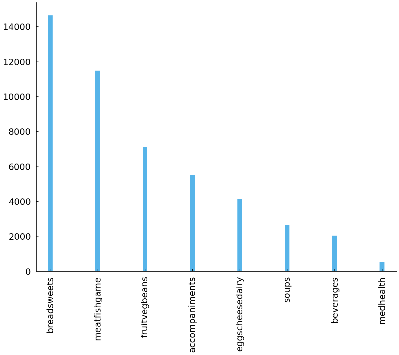
df['recipe_class'].value_counts()
breadsweets        14630
meatfishgame       11477
fruitvegbeans       7085
accompaniments      5495
eggscheesedairy     4150
soups               2631
beverages           2031
medhealth            533
Name: recipe_class, dtype: int64
The table shows that “bread and sweets” is the most common recipe category, followed by
recipes for “meat, fish, and game”, and so on and so forth. Plotting these values is as
easy as calling the method plot() on top of the Series object returned by
value_counts(). In the code block
below, we set the argument kind to 'bar' to create a bar plot. The color of all bars
is set to the first default color. To make the plot slightly more attractive, we set the
width of the bars to 0.1:
df['recipe_class'].value_counts().plot(kind='bar', color="C0", width=0.1);
findfont: Font family ['sans-serif'] not found. Falling back to DejaVu Sans.
findfont: Generic family 'sans-serif' not found because none of the following families were found: "Roboto Condensed Regular"
We continue our exploration of the data. Before we can address our first research question about popularity shifts of ingredients, it is important to get an impression of how the data are distributed over time. The following lines of code plot the number of recipes for each attested year in the collection. Pay close attention to the comments following the hashtags:
import matplotlib.pyplot as plt

grouped = df.groupby('date')  # group all rows from the same year
recipe_counts = grouped.size()  # compute the size of each group
recipe_counts.plot(style='o', xlim=(1810, 1930))  # plot the group size
plt.ylabel("number of recipes")  # add a label to the Y-axis
plt.xlabel("year of publication") # add a label to the X-axis
Text(0.5, 0, 'year of publication')
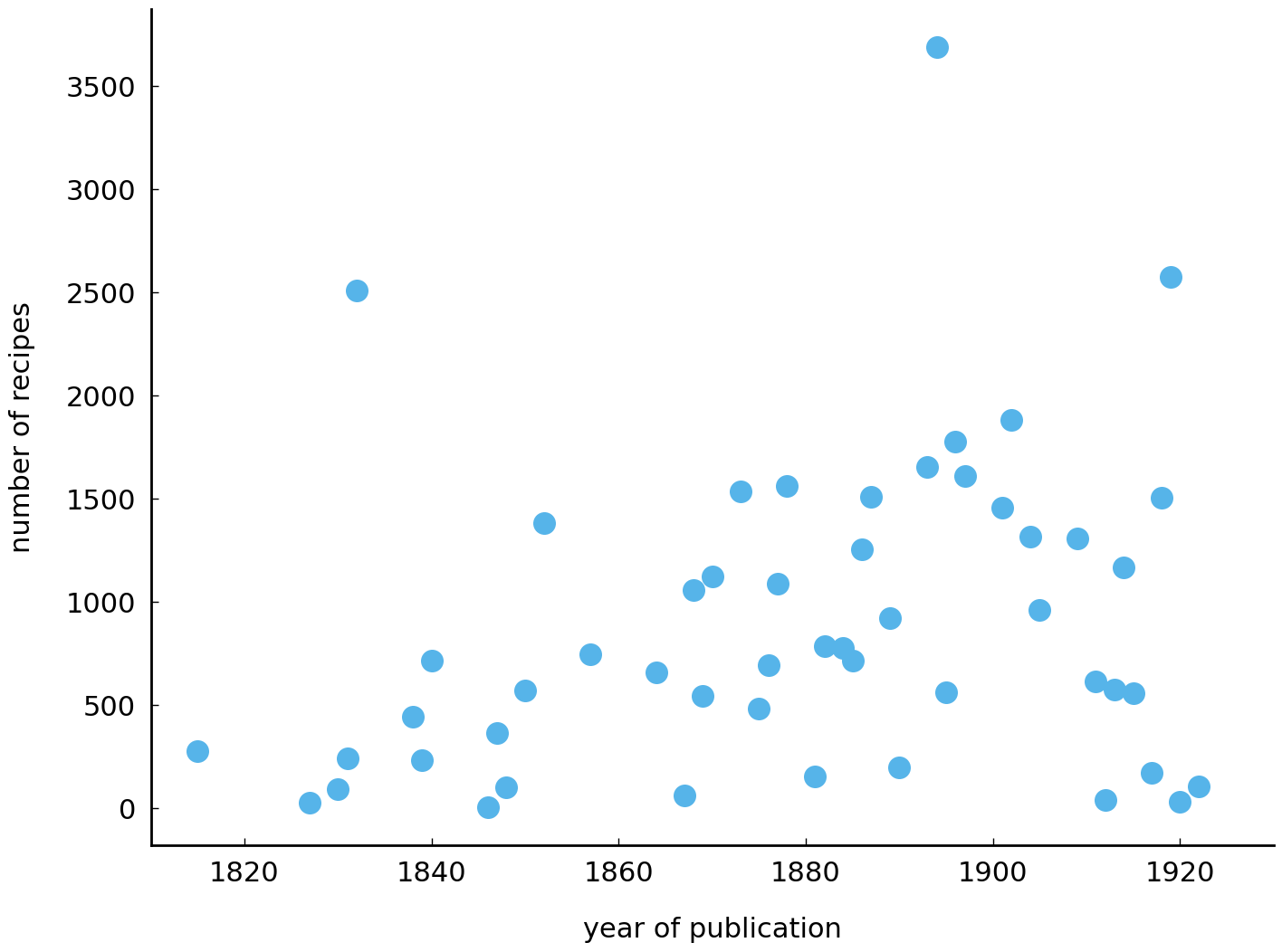
Here, groupby() groups all rows from the same year into separate data frames. The size
of these groups (i.e., how many recipes are attested in a particular year), then, is
extracted by calling size(). Finally, these raw counts are plotted by
calling plot(). (Note that we set the style to 'o' to plot points instead of a
line.) While a clear trend cannot be discerned, a visual inspection of the graph seems to
hint at a slight increase in the number of recipes over the years—but further analyses
will have to confirm whether any of the trends we might discern are real.
Taste Trends in Culinary US History#
Having explored some rudimentary aspects of the dataset, we can move on to our first
research question: can we observe some trends in the use of certain ingredients over time?
The column “ingredients” provides a list of ingredients per recipe, with each ingredient
separated by a semicolon. We will transform these ingredient lists into a slightly more
convenient format, allowing us to more easily plot their usage frequency over time. Below,
we first split the ingredient strings into actual Python lists using
str.split(';'). Next, we group all recipes from the same year and merge their
ingredient lists with sum(). By applying Series.value_counts() in the next step, we
obtain frequency distributions of ingredients for each year. In order to make sure that
any frequency increase of ingredients is not simply due to a higher number of recipes, we
should normalise the counts by dividing each ingredient count by the number of attested
recipes per year. This is done in the last line.
# split ingredient strings into lists
ingredients = df['ingredients'].str.split(';')
# group all rows from the same year
groups = ingredients.groupby('date')
# merge the lists from the same year
ingredients = groups.sum()
# compute counts per year
ingredients = ingredients.apply(pd.Series.value_counts)
# normalise the counts
ingredients = ingredients.divide(recipe_counts, 0)
These lines of code are quite involved. But don’t worry: it is not necessary to understand
all the details at this point (it will get easier after completing chapter
Processing Tabular Data). The resulting data frame consists of rows representing a
particular year in the collection and columns representing individual ingredients (this
format will be revisited in chapter Exploring Texts using the Vector Space Model). This allows us to
conveniently extract, manipulate, and plot time series for individual ingredients. Calling
the head() method allows us to inspect the first five rows of the new data frame:
ingredients.head()
| butter | salt | water | flour | nutmeg | pepper | sugar | lemon | mace | egg | ... | tomato in hot water | farina cream | pearl grit | chicken okra | tournedo | avocado | rock cod fillet | perch fillet | lime yeast | dried flower | |
|---|---|---|---|---|---|---|---|---|---|---|---|---|---|---|---|---|---|---|---|---|---|
| date | |||||||||||||||||||||
| 1803 | 0.570796 | 0.435841 | 0.409292 | 0.351770 | 0.272124 | 0.267699 | 0.205752 | 0.205752 | 0.188053 | 0.150442 | ... | NaN | NaN | NaN | NaN | NaN | NaN | NaN | NaN | NaN | NaN |
| 1807 | 0.357374 | 0.349839 | 0.395048 | 0.219591 | 0.132400 | 0.194833 | 0.274489 | 0.104413 | 0.134553 | 0.177610 | ... | NaN | NaN | NaN | NaN | NaN | NaN | NaN | NaN | NaN | NaN |
| 1808 | 0.531401 | 0.371981 | 0.391304 | 0.352657 | 0.260870 | 0.149758 | 0.396135 | 0.115942 | 0.140097 | 0.294686 | ... | NaN | NaN | NaN | NaN | NaN | NaN | NaN | NaN | NaN | NaN |
| 1815 | 0.398551 | 0.315217 | 0.322464 | 0.431159 | 0.152174 | 0.083333 | 0.387681 | 0.018116 | 0.036232 | 0.347826 | ... | NaN | NaN | NaN | NaN | NaN | NaN | NaN | NaN | NaN | NaN |
| 1827 | NaN | 0.066667 | 0.600000 | NaN | 0.033333 | 0.033333 | 0.400000 | 0.200000 | NaN | 0.033333 | ... | NaN | NaN | NaN | NaN | NaN | NaN | NaN | NaN | NaN | NaN |
5 rows × 3532 columns
Using the ingredient data frame, we will first explore the usage of three ingredients, which have been discussed by different culinary historians: tomatoes, baking powder, and nutmeg (see, e.g., Kraig [2013]). Subsequently, we will use it to employ a data-driven exploration technique to automatically find ingredients that might have undergone some development over time.
Let us start with tomatoes. While grown and eaten throughout the nineteenth century, tomatoes did not feature often in early nineteenth century American dishes. One of the reasons for this distaste was that tomatoes were considered poisonous, hindering their widespread diffusion in the early 1900s. Over the course of the nineteenth century, tomatoes only gradually became more popular until, around 1880, Livingston created a new tomato breed which transformed the tomato into a commercial crop and started a true tomato craze. At a glance, these developments appear to be reflected in the time series of tomatoes in the Feeding America cookbook collection:
ax = ingredients['tomato'].plot(style='o', xlim=(1810, 1930))
ax.set_ylabel("fraction of recipes")
ax.set_xlabel("year of publication");
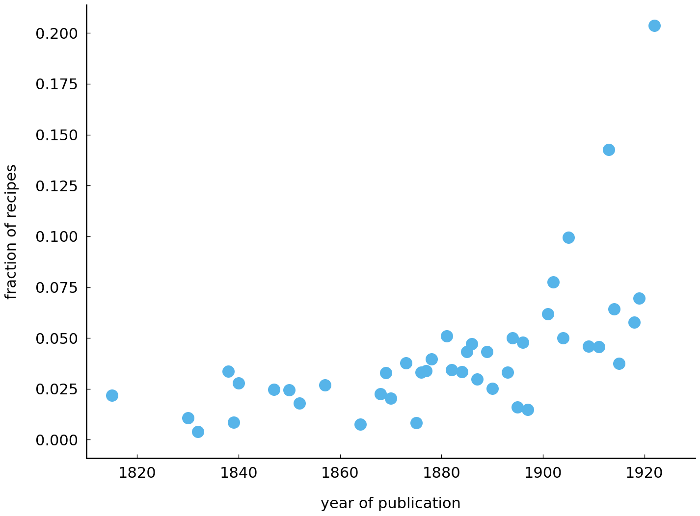
Here, ingredients['tomato'] selects the column “tomato” from our ingredients data
frame. The column values, then, are used to draw the time series graph. In order to
accentuate the rising trend in this plot, we can add a “least squares line” as a
reference. The following code block implements a utility function, plot_trend(), which
enhances our time series plots with such a trend line:
import scipy.stats

def plot_trend(column, df, line_color='grey', xlim=(1810, 1930)):
    slope, intercept, _, _, _ = scipy.stats.linregress(
        df.index, df[column].fillna(0).values)
    ax = df[column].plot(style='o', label=column)
    ax.plot(df.index, intercept + slope * df.index, '--',
             color=line_color, label='_nolegend_')
    ax.set_ylabel("fraction of recipes")
    ax.set_xlabel("year of publication")
    ax.set_xlim(xlim)
plot_trend('tomato', ingredients)
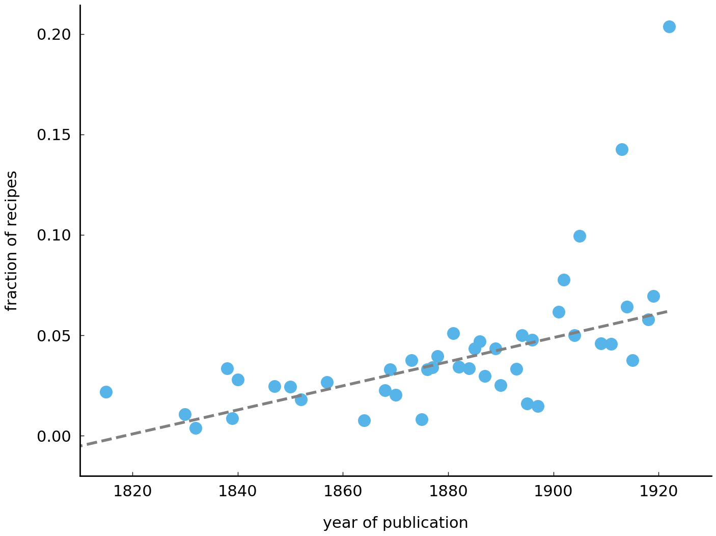
The last lines of the function plot_trend() plots the trend line. To do that, it uses
Python’s plotting library, Matplotlib, which we imported a while back in this chapter. The plot
illustrates why it is often useful to add a trend line. While the individual data points
seem to suggest a relatively strong frequency increase, the trend line in fact hints at a
more gradual, conservative increase.
Another example of an ingredient that went through an interesting development is baking powder. The plot below shows a rapid increase in the usage of baking powder around 1880, just forty years after the first modern version of baking powder was discovered by the British chemist Alfred Bird. Baking powder was used in a manner similar to yeast, but was deemed better because it acts more quickly. The benefits of this increased cooking efficiency is reflected in the rapid turnover of baking powder at the end of the 19th century:
plot_trend('baking powder', ingredients)
plot_trend('yeast', ingredients)
plt.legend();  # add a legend to the plot
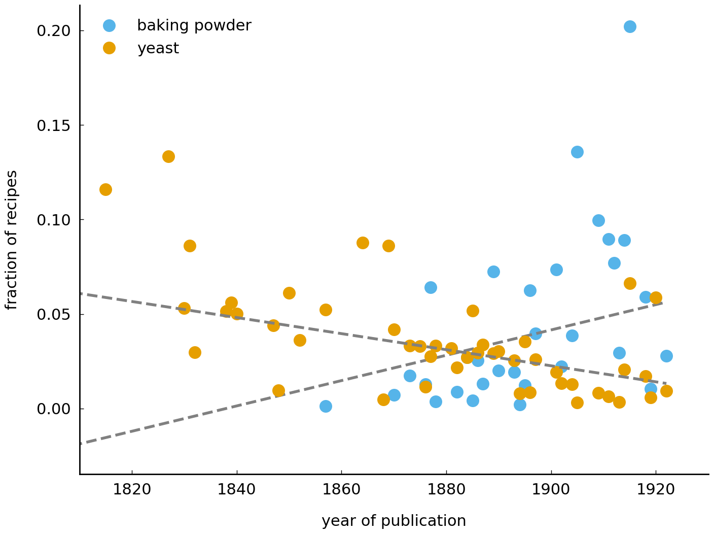
The plot shows two clear trends: (i) a gradual decrease of yeast use in the early nineteenth century, which (ii) is succeeded by the rise of baking powder taking over the position of yeast in American kitchens.
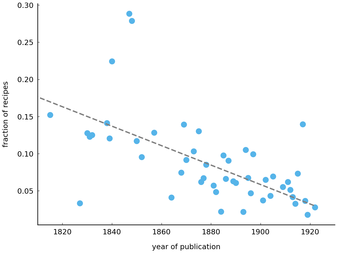
As a final example, we explore the use of nutmeg. Nutmeg, a relatively small brown seed, is an interesting case as it has quite a remarkable history. The seed was deemed so valuable that, in 1667 at the Treaty of Breda, the Dutch were willing to trade Manhattan for the small Run Island (part of the Banda Islands of Indonesia), and subsequently, in monopolizing its cultivation, the local people of Run were brutally slaughtered by the Dutch colonists. Nutmeg was still extremely expensive in the early nineteenth century, while at the same time highly popular and fashionable in American cooking. However, over the course of the nineteenth century, nutmeg gradually fell out of favor in the American kitchen, giving room to other delicate (and pricy) seasonings. The plot below displays a clear decay in the usage of nutmeg in nineteenth century American cooking, which is in line with these narrative descriptions in culinary history:
plot_trend('nutmeg', ingredients)
While it is certainly interesting to visualize and observe the trends described above, the examples given above are well-known cases from the literature. Yet, the real interesting purpose of exploratory data analysis is to discover new patterns and regularities, revealing new questions and hypotheses. As such, adopting a method that does not rely on pre-existing knowledge on the subject matter would be more interesting for an exploratory analysis.
One such method is, for instance, measuring the “distinctiveness” or “keyness” of certain
words in a collection. We could, for example, measure which ingredients are distinctive
for recipes stemming from northern states of the United States versus those originating from southern
states. Similarly, we may be interested in what distinguishes the post-Civil War era from
before the war in terms of recipe ingredients. Measuring “distinctiveness” requires a
definition and formalization of what distinctiveness means. A well-known and commonly used
definition for measuring keyness of words is Pearson’s \(\chi^2\) test statistic, which
estimates how likely it is that some observed difference (e.g., the usage frequency of
tomatoes before and after the Civil War) is the result of chance. The machine learning
library scikit-learn implements this test statistic in
the function chi2(). Below, we demonstrate how to use this function to find ingredients
distinguishing the pre-Civil War era from postwar times:
from sklearn.feature_selection import chi2

# Transform the index into a list of labels, in which each label
# indicates whether a row stems from before or after the Civil War:
labels = ['Pre-Civil War' if year < 1864 else 'Post-Civil War' for year in ingredients.index]
# replace missing values with zero (.fillna(0)),
# and compute the chi2 statistic:
keyness, _ = chi2(ingredients.fillna(0), labels)
# Turn keyness values into a Series, and sort in descending order:
keyness = pd.Series(keyness, index=ingredients.columns).sort_values(ascending=False)
Inspecting the head of the keyness series gives us an overview of the n ingredients that
most sharply distinguish pre- and postwar times:
keyness.head(n=10)
nutmeg           1.072078
rice water       1.057412
loaf sugar       1.057213
mace             0.955977
pearlash         0.759318
lemon peel       0.694849
baking powder    0.608744
soda             0.589730
vanilla          0.533900
gravy            0.453685
dtype: float64
The \(\chi^2\) test statistic identifies “nutmeg” as the ingredient most clearly distinguishing the two time frames (in line with its popularity decline descibed above and in the literature). “Mace” is a spice made from the reddish seed of the nutmeg seed, and as such, it is no surprise to also find it listed high in the ranking of most distinctive ingredients. Another interesting pair is “baking powder” and “pearlash”. We previously related the decay of “yeast” to the rise of “baking powder”, but did not add “pearlash” to the picture. Still, it is reasonable to do so, as pearlash (or potassium carbonate) can be considered the first chemical leavener. When combined with an acid (e.g., citrus), pearlash produces a chemical reaction with a carbon dioxide by-product, adding a lightness to the product. The introduction of pearlash is generally attributed to the author of America’s first cookbook, the aforementioned Amelia Simmons.
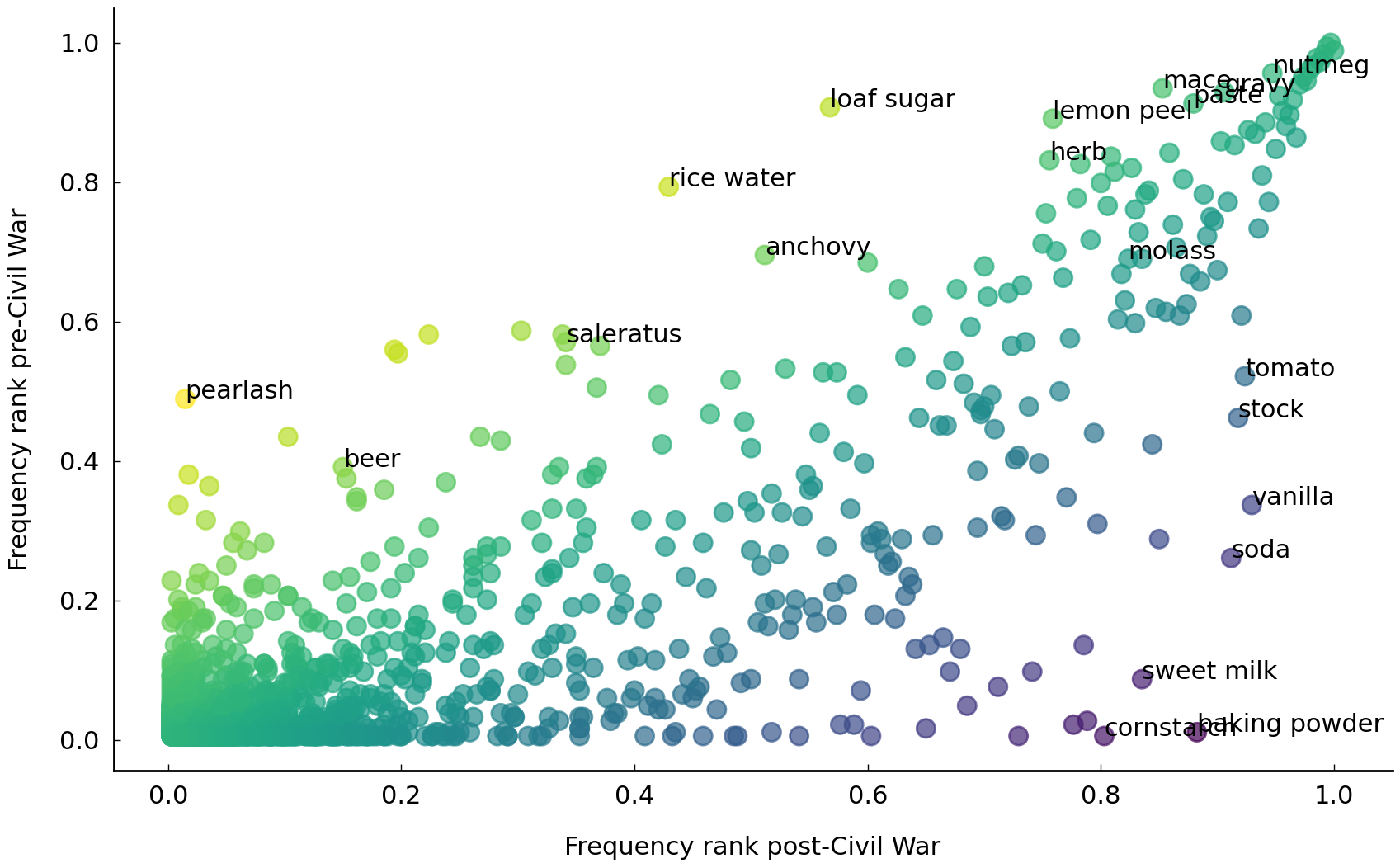
One thing that should be noted here is that, while \(\chi^2\) gives us an estimation of the keyness of certain ingredients, it does not tell us the direction of this effect, i.e., whether a particular ingredient is distinctive for one or both collections. Below, we will explore the direction of the effects by creating a simple, yet informative visualization (inspired by Kessler [2017]). The visualization is a simple scatterplot in which the X axis represents the frequency of an ingredient in the post-Civil War era and the Y axis represents the frequency prior to the war. Let us first create the plot; then we will explain how to read and interpret it.
# step 1: compute summed ingredient counts per year
counts = df['ingredients'].str.split(';').groupby(
    'date').sum().apply(pd.Series.value_counts).fillna(0)

# step 2: construct frequency rankings for pre- and postwar years
pre_cw = counts[counts.index < 1864].sum().rank(method='dense', pct=True)
post_cw = counts[counts.index > 1864].sum().rank(method='dense', pct=True)

# step 3: merge the pre- and postwar data frames
rankings = pd.DataFrame({'Pre-Civil War': pre_cw, 'Post-Civil War': post_cw})

# step 4: produce the plot
fig = plt.figure(figsize=(10, 6))
plt.scatter(rankings['Post-Civil War'], rankings['Pre-Civil War'],
            c=rankings['Pre-Civil War'] - rankings['Post-Civil War'],
            alpha=0.7)

# Add annotations of the 20 most distinctive ingredients
for i, row in rankings.loc[keyness.head(20).index].iterrows():
    plt.annotate(i, xy=(row['Post-Civil War'], row['Pre-Civil War']))

plt.xlabel("Frequency rank post-Civil War")
plt.ylabel("Frequency rank pre-Civil War");
These lines of code are quite complicated. Again, don’t worry if you don’t understand
everything. You don’t need to. Creating the plot involves the following four steps. First,
we construct a data frame with unnormalized ingredient counts, which lists how often the
ingredients in the collection occur in each year (step 1). In the second step, we split
the counts data frame into a pre- and postwar data frame, compute the summed ingredient
counts for each era, and, finally, create ranked lists of ingredients based on their
summed counts. In the third step, the pre- and postwar data frames are merged into the
rankings data frame. The remaining lines (step 4) produce the actual plot, which
involves a call to pyplot.scatter() for creating a scatter
plot, and a loop to annotate the plot with labels for the top twenty most distinctive
ingredients (pyplot.annotate()).
The plot should be read as follows: in the top right, we find ingredients frequently used both before and after the war. Infrequent ingredients in both eras are found in the bottom left. The more interesting ingredients are found near the top left and bottom right corners. These ingredients are either used frequently before the war but infrequently after the war (top left), or vice versa (bottom right). Using this information, we can give a more detailed interpretation to the previously computed keyness numbers, and observe that ingredients like pearlash, saleratus, rice water and loaf sugar are distinctive for pre-war times, while olive oil, baking powder, and vanilla are distinctive for the more modern period. We leave it up to you to experiment with different time frame settings as well as highlighting larger numbers of key ingredients. The brief analysis and techniques presented here serve to show the strength of performing simple exploratory data analyses, with which we can assess and confirm existing hypotheses, and potentially raise new questions and directions for further research.
America’s Culinary Melting Pot#
Now that we have a better picture of a number of important changes in the use of cooking ingredients, we move on to our second research question: Can we observe the influence of immigration waves in the Feeding America cookbook collection? The nineteenth century United States has witnessed multiple waves of immigration. While there were relatively few immigrants in the first three decades, large-scale immigration started in the 1830s with people coming from Britain, Ireland, and Germany. Other immigration milestones include the 1848 Treaty of Guadalupe Hidalgo, providing US citizenship to over 70,000 Mexican residents, and the “new immigration” starting around the 1880s, in which millions of (predominantly) Europeans took the big trip to the United States (see, e.g., Themstrom et al. [1980]). In this section, we will explore whether these three waves of immigration have left their mark in the Feeding America cookbook collection.
The compilers of the Feeding America dataset have provided high-quality annotations for
the ethnic origins of a large number of recipes. This information is stored in the
“ethnicgroup” column of the df data frame, which we defined in the previous section.
We will first investigate to what extent these annotations can help us to identify
(increased) influences of foreign cooking traditions. To obtain an overview of the
different ethnic groups in the data as well as their distibution, we construct a frequency
table using the method value_counts():
df['ethnicgroup'].value_counts(dropna=False).head(10)
NaN         41432
jewish       3418
creole        939
french        591
oriental      351
italian       302
english       180
german        153
spanish       123
chinese        66
Name: ethnicgroup, dtype: int64
Recipes from unknown origin have the value NaN (standing for “Not a Number”), and by
default, value_counts() leaves out NaN values. However, it would be interesting to gain
insight into the number of recipes of which the origin is unknown or unclassified. To include these
recipes in the overview, the parameter dropna was set to False. It is clear from the
table above that the vast majority of recipes provides no information about their ethnic
group. The top known ethnicities include “Jewish”, “Creole”, “French” and so on. As a
simple indicator of increasing foreign cooking influence, we would expect to observe an
increase over time in the number of unique ethnic groups. This expectation appears to be
confirmed by the graph constructed below, which displays the average number of different
ethnic groups attested each year:
grouped = df.groupby(level='date')
# compute the number of unique ethnic groups per year,
# divided by the number of books
n_groups = grouped['ethnicgroup'].nunique() / grouped['book_id'].nunique()
n_groups.plot(style='o')

# add a least squares line as reference
slope, intercept, _, _, _ = scipy.stats.linregress(
    n_groups.index, n_groups.fillna(0).values)

# create the plot
plt.plot(
    n_groups.index, intercept + slope * n_groups.index, '--', color="grey")
plt.xlim(1810, 1930)
plt.ylabel("Average number of ethnic groups")
plt.xlabel("Year of publication");
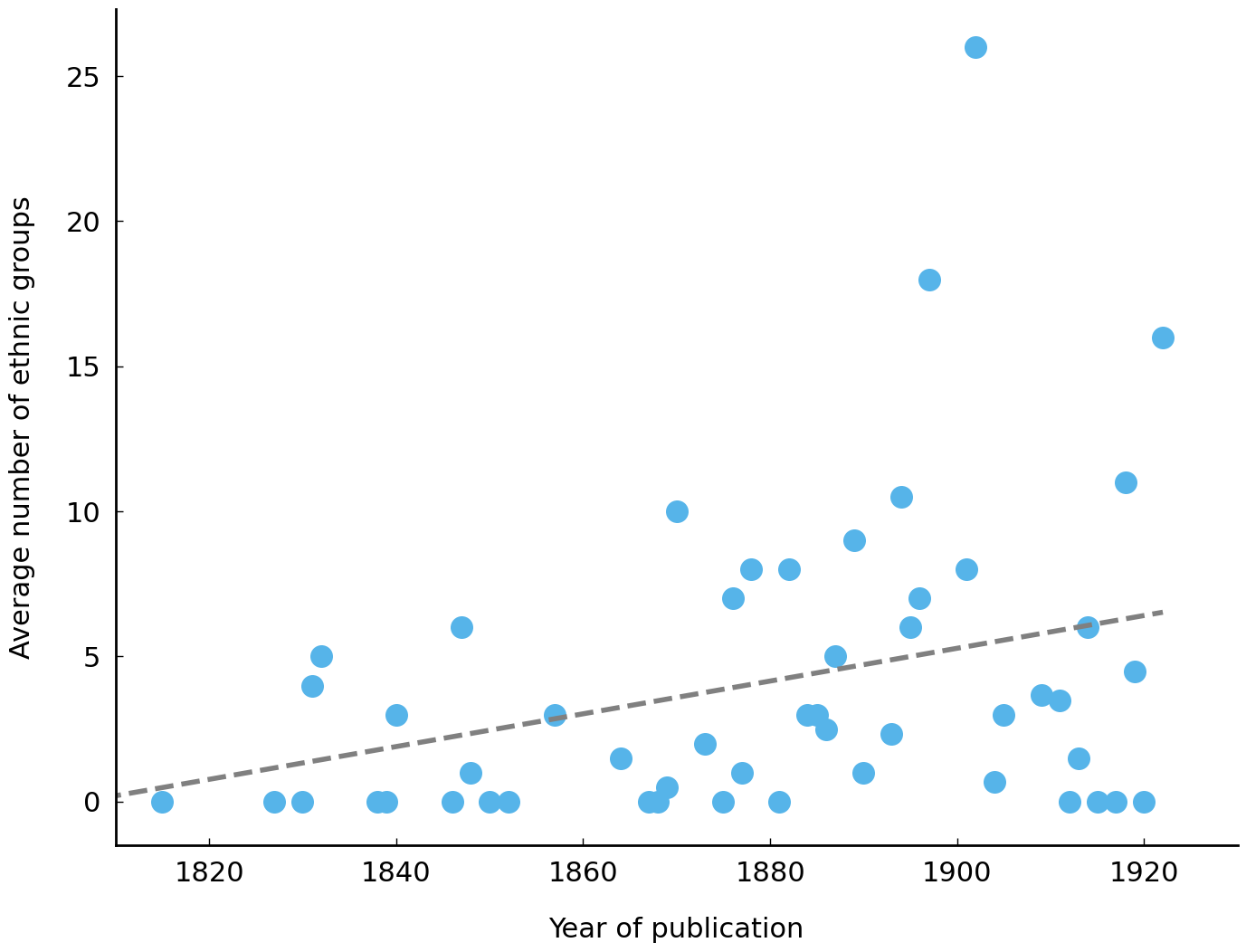
The graph shows a gradual increase in the number of ethnic groups per year, with (small) peaks around 1830, 1850, 1880, and 1900. It is important to stress that these results do not conclusively support the hypothesis of increasing foreign influence in American cookbooks, because it may very well reflect an artifact of our relatively small cookbook dataset. However, the purpose of exploratory data analysis is not to provide conclusive answers, but to point at possibly interesting paths for future research.
To obtain a more detailed description of the development sketched above, let us try to zoom in on some of the foreign culinary contributions. We will employ a similar strategy as before and use a keyness analysis to find ingredients distinguishing ethnically annotated from ethnically unannotated recipes. Here, “keyness” is defined slightly differently as the difference between two frequency ranks. Consider the plot below and the different coding steps in the following code block:
# step 1: add a new column indicating for each recipe whether
#         we have information about its ethnic group
df['foreign'] = df['ethnicgroup'].notnull()

# step 2: construct frequency rankings for foreign and general recipes
counts = df.groupby('foreign')['ingredients'].apply(
    ';'.join).str.split(';').apply(pd.Series.value_counts).fillna(0)

foreign_counts = counts.iloc[1].rank(method='dense', pct=True)
general_counts = counts.iloc[0].rank(method='dense', pct=True)

# step 3: merge the foreign and general data frames
rankings = pd.DataFrame({'foreign': foreign_counts, 'general': general_counts})

# step 4: compute the keyness of ingredients in foreign recipes
#         as the difference in frequency ranks
keyness = (rankings['foreign'] - rankings['general']).sort_values(ascending=False)

# step 5: produce the plot
fig = plt.figure(figsize=(10, 6))
plt.scatter(rankings['general'], rankings['foreign'],
            c=rankings['foreign'] - rankings['general'],
            alpha=0.7)

for i, row in rankings.loc[keyness.head(10).index].iterrows():
    plt.annotate(i, xy=(row['general'], row['foreign']))

plt.xlabel("Frequency rank general recipes")
plt.ylabel("Frequency rank foreign recipes");
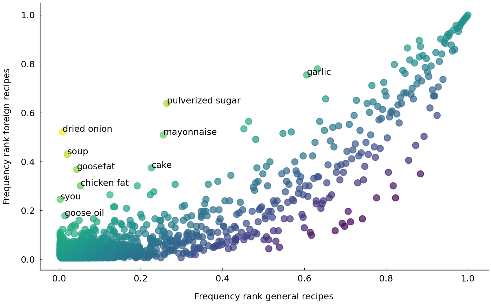
The plot is another scatter plot, highlighting a number of ingredients that are distinctive for recipes annotated for ethnicity. Some notable ingredients are “olive oil”, “garlic”, “syou”, and “mayonnaise”. “Olive oil” and “garlic” were both likely imported by Mediterranean immmigrants, while “syou” (also called soye) was brought in by Chinese newcomers. Finally, while “mayonnaise” is a French invention, its introduction in the United States is generally attributed to Richard Hellmann who emigrated from Germany in 1903 to New York City. His Hellmann’s Mayonnaise with its characteristic blue ribbon jars became highly popular during the interbellum and still is a popular brand in the United States today.
In sum, the brief analysis presented here warrants further investigating the connection between historical immigration waves and changing culinary traditions in nineteenth century America. It was shown that over the course of the nineteenth century we see a gradual increase in the number of unique recipe origins, which coincides with important immigration milestones.
Further Reading#
In this chapter, we have presented the broad topic of exploratory data analysis, and applied it to a collection of historical cookbooks from 19th century America. The analyses presented above served to show that computing basic statistics and producing elementary visualizations are important for building intuitions about a particular data collection, and, when used strategically, can aid the formulation of new hypotheses and research questions. Being able to perform such exploratory finger exercises is a crucial skill for any data analyst as it helps to improve and harness data cleaning, data manipulation and data visualization skills. Exploratory data analysis is a crucial first step to validate certain assumptions about and identify particular patterns in data collections, which will inform the understanding of a research problem and help to evaluate which methodologies are needed to solve that problem. In addition to (tentatively) answering a number of research questions, the chapter’s exploratory analyses have undoubtedly left many important issues unanswered, while at the same time raising various new questions. In the chapters to follow, we will present a range of statistical and machine learning models with which these issues and questions can be addressed more systematically, rigorously, and critically. As such, the most important guide for further reading we can give in this chapter is to jump into the subsequent chapters.
Exercises#
Easy#
Load the cookbook data set, and extract the “region” column. Print the number of unique regions in the data set.
Using the same “region” column, produce a frequency distribution of the regions in the data.
Create a bar plot of the different regions annotated in the dataset.
Moderate#
Use the function
plot_trend()to create a time series plot for three or more ingredients of your own choice.Go back to section Taste Trends in Culinary US History. Create a bar plot of the ten most distinctive ingredients for the pre- and postwar era using as keyness measure the Pearson’s \(\chi^2\) test statistic.
With the invention of baking powder, cooking efficiency went up. Could there be a relationship between the increased use of baking powder and the number of recipes describing cakes, sweets, and bread? (The latter recipes have the value
"breadsweets"in therecipe_classcolumn in the original data.) Produce two time series plots: one for the absolute number of recipes involving baking powder as ingredient, and a second plotting the absolute number"breadsweets"recipes over time.
Challenging#
Use the code to produce the scatter plot from section Taste Trends in Culinary US History, and experiment with different time frame settings to find distinctive words for other time periods. For example, can you compare twentieth-century recipes to nineteenth-century recipes?
Adapt the scatter plot code from section America’s Culinary Melting Pot to find distinctive ingredients for two specific ethnic groups. (You could, for instance, contrast typical ingredients from the Jewish cuisine with those from the Creole culinary tradition.) How do these results differ from the ethnicity plot we created before? (Hint: For this exercise, you could simply adapt the very final code block of the chapter and use the somewhat simplified keyness measure proposed there.)
Use the “region” column to create a scatter plot of distinctive ingredients in the northeast of the United States versus the ingredients used in the midwest. To make things harder on yourself, you could use Pearson’s \(\chi^2\) test statistic as a keyness measure.