Introduction to Probability
Contents
Introduction to Probability#
Probabilities are used in everyday speech to describe uncertain events and degrees of belief about past and future states of affairs. A newspaper writer might, for example, write about the likely outcome of an election held the following day, or a student might talk about the their chance of having received a passing score on a test they just completed. This chapter discusses the use of probabilities in the context of one account of what it means to learn from experience: Bayesian inference. Bayesian inference provides both (1) an interpretation of probabilities, and (2) a prescription for how to update probabilities in light of evidence (i.e., how to learn from experience). Both these items are important. Treating probability statements as statements about degree of belief is useful whenever we need to communicate or compare our judgment of the credibility of a hypothesis (or model) with the judgments of others, something that happens all the time in the course of historical research. And having a method of learning from evidence is important because it is useful to be able to assess how evidence, in particular new evidence, supports or undermines theories.
The goal of this chapter is to illustrate Bayesian inference as applied to the task of authorship attribution. The chapter begins with an informal discussion of probabilities and Bayesian inference. A fictional case of authorship attribution is used to prepare readers for a full treatment later in the chapter. This introduction is followed by a formal characterization of probabilities and Bayes’s rule. The introduction should leave readers familiar with the basic vocabulary encountered in data analysis in the humanities and allied social sciences. This formal introduction is followed by a return to the task of authorship attribution. The bulk of the chapter is devoted to a detailed case study examining the classic case of disputed authorship of several essays in The Federalist Papers.
One note of warning: this chapter does not offer a complete introduction to probability. An appreciation of the material in this chapter requires some familiarity with standard discrete probability distributions. This kind of familiarity is typically obtained in an introductory mathematics or statistics course devoted to probability. We discuss appropriate preliminary readings at the end of this chapter. For many kinds of humanities data, one specific discrete probability distribution—one featured in this chapter—is of great importance: the negative binomial distribution. Indeed, facility with the negative binomial distribution counts as an essential skill for anyone interested in modeling word frequencies in text documents. The negative binomial distribution is the simplest probability distribution which provides a plausible model of word frequencies observed in English-language documents [Church and Gale, 1995]. The only kinds of words which can be credibly modeled with more familiar distributions (e.g., normal, binomial, or Poisson) are those which are extremely frequent or vanishingly rare.
Uncertainty and Thomas Pynchon#
To motivate the Bayesian task of learning from evidence, consider the following scenario. It has been suggested that Thomas Pynchon, a well-known American novelist, may have written under a pseudonym during his long career (e.g., Winslow [2015]). Suppose the probability of a work of literary fiction published between 1960 and 2010 being written by Thomas Pynchon (under his own name or under a pseudonym) is 0.001 percent, i.e., 1 in 100,000. Suppose, moreover, that a stylometric test exists which is able to identify a novel as being written by Pynchon 90 percent of the time (i.e., the true positive rate—“sensitivity” in some fields—equals 0.9). One percent of the time, however, the test mistakenly attributes the work to Pynchon (i.e., the false positive rate equals 0.01). In this scenario, we assume the test works as described; we might imagine Pynchon himself vouches for the accuracy of the test or that the test invariably exhibits these properties over countless applications. Suppose a novel (written by someone other than Pynchon) published in 2010 tests positive on the stylometric test of Pynchon authorship. What is the probability that the novel was penned by Pynchon?
One answer to this question is provided by Bayes’s rule, which is given below and whose justification will be addressed shortly:
where \(\positive\) indicates the event of the novel testing positive and \(\Pynchon\) indicates the event of the novel having been written by Pynchon. The preceding paragraph provides us with values for all the quantities on the right-hand side of the equation, where we have used the expression \(\Pr(A)\) to indicate the probability of the event \(A\) occurring.
pr_pynchon = 0.00001
pr_positive = 0.90
pr_false_positive = 0.01
print(pr_positive * pr_pynchon / (pr_positive * pr_pynchon +
                                  pr_false_positive * (1 - pr_pynchon)))
0.000899199712256092
Bayes’ rule produces the following answer: the probability that Pynchon is indeed the author of the novel given a positive test is roughly one tenth of one percent. While this is considerably higher than the baseline of one hundredth of one percent, it seems underwhelming given the stated accuracy (90 percent) of the test.
Note
A less opaque rendering of this rule relies on the use of natural frequencies. Ten out of every 1,000,000 novels published between 1960 and 2010 are written by Pynchon. Of these 10 novels, 9 will test positive as Pynchon novels. Of the remaining 999,990 novels not written by Pynchon, approximately 10,000 will test positive as Pynchon novels. Suppose you have a small sample of novels which have tested positive, how many of the novels are actually written by Pynchon? The answer is the ratio of true positives to total positives, or \(9 / 10009 \approx 0.0009\), or 0.09 percent. So the conclusion is the same. Despite the positive test, the novel in question remains unlikely to be a Pynchon novel.
This example illustrates the essential features of Bayesian learning: we begin with a prior probability, a description of how likely a novel published between 1960 and 2010 is a novel by Pynchon, and then update our belief in light of evidence (a positive test result using a stylometric test), and arrive at a new posterior probability. While we have yet to address the question of why the use of this particular procedure—with its requirement that degree of belief be expressed as probabilities between 0 and 1—deserves deference, we now have at least a rudimentary sense about what Bayesian learning involves.
This extended motivating example prepares us for the case study at the center of this chapter: the disputed authorship of several historically significant essays by two signers of the United States Constitution: Alexander Hamilton and James Madison. That this case study involves, after Roberto Busa’s encounters with Thomas Watson, the best known instance of humanities computing avant la lettre will do no harm either. The case study will, we hope, make abundantly clear the challenge Bayesian inference addresses: the challenge of describing—to at least ourselves and potentially to other students or researchers—how observing a piece of evidence changes our prior beliefs.
Probability#
This section provides a formal introduction to probabilities and their role in Bayesian inference. Probabilities are the lingua franca of the contemporary natural and social sciences; their use is not without precedent in the humanities research either, as the case study in this chapter illustrates. Authorship attribution is a fitting site for an introduction to using probabilities in historical research because the task of authorship attribution has established contours and involves using probabilities to describe beliefs about events in the distant past—something more typical of historical research than other research involving the use of probabilities.
Probabilities are numbers between 0 and 1. For our purposes—and in Bayesian treatments of probability generally—probabilities express degree of belief. For example, a climatologist would use a probability (or a distribution over probabilities) to express their degree of belief in the hypothesis that the peak temperature in Germany next year will be higher than the previous year. If one researcher assigns a higher probability to the hypothesis than another researcher, we say that the first researcher finds (or tends to find) the hypothesis more credible, just as we would likely say in a less formal discussion.
For concreteness, we will anchor our discussion of probabilities (degrees of belief) in a specific case. We will discuss probabilities that have been expressed by scholars working on a case of disputed authorship. In 1964, Frederick Mosteller (1916–2006) and David Wallace (1928–2017) investigated the authorship of twelve disputed essays which had been published under a pseudonym in New York newspapers between 1787 and 1788. The dispute was between two figures well-known in the history of the colonization of North America by European settlers: Alexander Hamilton and James Madison. Each claimed to be the sole author of all twelve essays. These twelve essays were part of a larger body of eightyfive essays known collectively as The Federalist Papers. The essays advocated ratification of the United States Constitution. In the conclusion of their study, Mosteller and Wallace offer probabilities to describe their degrees of belief about the authorship of each of the twelve essays. For example, they report that the probability Federalist No. 62 is written by Madison is greater than 99.9 percent (odds of 300,000 to 1) while the probability Federalist No. 55 is written by Madison is 99 percent (100 to 1). In the present context, it is useful to see how Mosteller expresses their conclusion: “Madison is extremely likely, in the sense of degree of belief, to have written the disputed Federalist essays, with the possible exception of No. 55, and there our evidence is weak; suitable deflated odds are 100 to 1 for Madison” (Mosteller [1987], 139).
It should now be clear what probabilities are. It may not, however, be entirely clear what problem the quantitative description of degree of belief solves. What need is there, for example, to say that I believe that it will rain tomorrow with probability 0.8 when I might just as well say, “I believe it will likely rain tomorrow”? Or, to tie this remark to the present case, what is gained by saying that Madison is very likely the author of Federalist No. 62 versus saying that the odds favoring Madison’s authorship of the essay is 300,000 to 1? Those suspicious of quantification tout court might consider the following context as justification for using numbers to make fine distinctions about degrees of belief. In modern societies, we are familiar with occasions where one differentiates between various degrees of belief. The legal system provides a convenient source of examples. Whether you are familiar with judicial proceedings in a territory making use of a legal system in the common law tradition (e.g., United States) or a legal system in the civil law tradition (e.g., France), the idea that evidence supporting conviction must rise to a certain level should be familiar [Clermont and Sherwin, 2002]. If you are called to serve on a citizen jury (in a common law system) or called to arbitrate a dispute as a judge (in a civil law system), it is likely not sufficient to suspect that, say, Jessie stole Riley’s bike; you will likely be asked to assess whether you are convinced that Jessie stole Riley’s bike “beyond a reasonable doubt”. Another classic example of a case where making fine gradations between degrees of belief would be useful involves the decision to purchase an insurance contract (e.g., travel insurance). An informed decision requires balancing (1) the cost of the insurance contract, (2) the cost arising if the event insured against comes to pass, and (3) the probability that the event will occur.
Note
Consistent discussion of probabilities in ordinary language is sufficiently challenging that there are attempts to standardize the terminology. Consider, for example, the Intergovernmental Panel on Climate Change’s guidance on addressing uncertainties:
Term |
Likelihood of the outcome |
Odds |
Log odds |
|---|---|---|---|
Virtually certain |
> 99% probability |
> 99 (or 99:1) |
> 4.6 |
Very likely |
> 90% probability |
> 9 |
> 2.2 |
Likely |
> 66% probability |
> 2 |
> 0.7 |
About as likely as not |
33 to 66% probability |
0.5 to 2 |
0 to 0.7 |
Unlikely |
< 33% probability |
< 0.5 |
< -0.7 |
Very unlikely |
< 10% probability |
< 0.1 |
< -2.2 |
Exceptionally unlikely |
< 1% probability |
< 0.01 |
< -4.6 |
Probability and degree of belief#
Probabilities are one among many ways of expressing degrees of belief using numbers. (Forms of the words “plausibility” and “credibility” will also be used to refer to “degree of belief”.) Are they a particularly good way? That is, do probabilities deserve their status as the canonical means of expressing degrees of belief? Their characteristic scale (0 to 1) has, at first glance, nothing to recommend it over alternative continuous scales (e.g., -2 to 2, 1 to 5, or \(-\infty\) to \(\infty\)). Why should we constrain ourselves to this scale when we might prefer our own particular—and perhaps more personally familiar—scale? Presently, reviewing products (books, movies, restaurants, hotels, etc.) in terms of a scale of 1 to 5 “stars” is extremely common. A scale of 0 to 1 is rarely used.
A little reflection will show that the scale used by probabilities has a few mathematical properties that align well with a set of minimal requirements for deliberation involving degrees of belief. For example, the existence of a lower bound, \(0\), is consistent with the idea that, if we believe an event is impossible (e.g., an event which has already failed to occur), there can be no event in which we have a lower degree of belief. Similarly, the existence of an upper bound, \(1\), is consistent with the assumption that if we believe an event is certain (e.g., an event which has already occurred), there can be no event which is more plausible. Any bounded interval has this property; other intervals, such as zero to infinity, open intervals, or the natural numbers, do not.
The use of probabilities is also associated with a minimal set of rules, the “axioms of belief” or the “axioms of probability”, which must be followed when considering the aggregate probability of the conjunction or disjunction of events (Hoff [2009], 13–14; Casella and Berger [2001], 7–10). (The conjunction of events A and B is often expressed as “A or B”, the disjunction as “A and B”.) These rules are often used to derive other rules. For example, from the rule that all probabilities must be between 0 and 1, we can conclude that the probability of an aggregate event \(C\) that either event \(A\) occurs or event \(B\) occurs (often written as \(C = A \cup B\), where \(\cup\) denotes the union of elements in two sets) must also lie between 0 and 1.
Note
The axioms of probability, despite the appearance of the superficially demanding term “axiom”, only minimally constrain deliberations about events. Adhering to them is neither a mark of individual nor general obedience to a broader (universalizing) set of epistemological dispositions (e.g., “rationality”). The axioms demand very little. They demand, in essence, that we be willing to both bound and order our degrees of belief. They do not say anything about what our initial beliefs should be. If we are uncomfortable with, for example, ever saying ourselves (or entertaining someone else’s saying) that one event is more likely than another event (e.g., it is more likely that the writer of The Merchant of Venice was human than non-human), then the use of probabilities will have to proceed, if it proceeds at all, as a thought experiment. (A pessimistic view of the history of scientific claims of knowledge might figure in such a refusal to compare or talk in terms of degrees of belief.) Such a thought experiment would, however, find ample pragmatic justification: observational evidence and testimony in favor of the utility of probabilities is found in a range of practical endeavours, such as engineering, urban planning, and environmental science. And we need not explicitly endorse the axioms of probability in order to use them or to recommend their use.
When we use probabilities to represent degrees of belief, we use the following standard notation. The degree of belief that an event \(A\) occurs is \(\Pr(A)\). Events may be aggregated by conjunction or disjunction: \(A \textrm{ or } B\) is itself an event, as is \(A \textrm{ and } B\). The degree of belief that \(A\) occurs given that event \(B\) has already occurred is written \(\Pr(A|B)\). For a formal definition of “event” in this setting and a thorough treatment of probability, readers are encouraged to consult a text dedicated to probability, such as Grinstead and Snell [2012] or Hacking [2001].
Using this notation we can state the axioms of probability:
\(0 \le \Pr(A) \le 1\).
\(\Pr(A \textrm{ or } B) = \Pr(A) + \Pr(B)\) if \(A\) and \(B\) are mutually exclusive events.
\(\Pr(A \textrm{ and } B) = \Pr(B) \Pr(A|B)\).
Each of these axioms can be translated into reasonable constraints on the ways in which we are allowed to describe our degrees of belief. An argument for axiom 1 has been offered above. Axiom 2 implies that our degree of belief that one event in a collection of possible events will occur should not decrease if the set of possible events expands. (My degree of belief in rain occurring tomorrow must be less than or equal to my belief rain or snow will occur tomorrow.) Axiom 3 requires that the probability of a complex event be calculable when the event is decomposed into component “parts”. The rough idea is this: we should be free to reason about the probability of \(A\) and \(B\) both occurring by first considering the probability that \(B\) occurs and then considering the probability that \(A\) occurs given that \(B\) has occurred.
From the axioms of probability follows a rule, Bayes’s rule, which delivers a method of learning from observation. Bayes’s rule offers us a useful prescription for how our degree of belief in a hypothesis should change (or “update”) after we observe evidence bearing on the hypothesis. For example, we can use Bayes’s rule to calculate how our belief that Madison is the author of Federalist No. 51 (a hypothesis) should change after observing the number of times the word upon occurs in No. 51 (evidence). (Upon occurs much more reliably in Hamilton’s previous writings than in Madison’s.)
Bayes’s rule is remarkably general. If we can describe our prior belief about a hypothesis \(H\) as \(\Pr(H)\) (e.g., the hypothesis that Madison is the author of Federalist No. 51, \(\Pr(\textrm{Madison})\)), and describe how likely it would be to observe a piece of evidence \(E\) given that the hypothesis holds, \(\Pr(E|H)\) (e.g., the likelihood of observing upon given the hypothesis of Madison’s authorship, \(\Pr(\textrm{upon}|\textrm{Madison})\)), Bayes’s rule tells us how to “update” our beliefs about the hypothesis to arrive at our posterior degree of belief in the hypothesis, \(\Pr(H|E)\) (e.g., \(\Pr(\textrm{Madison}|\textrm{upon})\)), in the event that we indeed observe the specified piece of evidence. Formally, in a situation where there are \(K\) competing hypotheses, Bayes’ rule reads as follows,
where \(\Pr(H_k|E)\) is the probability of hypothesis \(k\) (\(H_k \in \mathcal{H}\)) given that evidence \(E\) is observed. Here we assume that the hypotheses are mutually exclusive and exhaust the space of possible hypotheses. In symbols we would write that the hypotheses \(H_k, k = 1, \ldots, K\) partition the hypothesis space: \(\cup_{k=1}^K H_k = \mathcal{H}\) and \(\cap_{k=1}^K H_k = \emptyset\). Bayes’ rule follows from the axioms of probability. A derivation of Bayes’ rule is provided in an appendix to this chapter (Appendix Bayes’s rule). A fuller appreciation of Bayes’s rule may be gained by considering its application to questions (that is, hypotheses) of interest. We turn to this task in the next section.
Example: Bayes’s Rule and Authorship Attribution#
In the case of authorship attribution of the disputed essays in The Federalist Papers, the space of hypotheses \(\mathcal{H}\) is easy to reason about: a disputed essay is written either by Hamilton or by Madison. There is also not much difficulty in settling on an initial “prior” hypothesis: the author of a disputed Federalist essay—we should be indifferent to the particular (disputed) essay—is as likely to be Hamilton as it is to be Madison. That is, the probability that a disputed essay is written by Hamilton (prior to observing any information about the essay) is equal to 0.5, the same probability which we would associate with the probability that the disputed essay is written by Madison. In symbols, if we use \(H\) to indicate the event of Hamilton being the author then \(\{ H, \neg H\}\) partitions the space of possible hypotheses. \(\Pr(H) = \Pr(\neg H) = 0.5\) expresses our initial indifference between the hypothesis that Hamilton is the author and the hypothesis that Madison (i.e., not Hamilton) is the author.
For this example, the evidence, given a hypothesis about the author, is the presence or absence of one or more occurrences of the word upon in the essay. This word is among several words which Mosteller and Wallace identify as both having a distinctive pattern in the essays of known authorship and being the kind of frequent “function” word widely accepted as having no strong connection between the subject matter addressed by a piece of writing. These function words are considered as promising subject-independent markers of authorial “style” (chapter chp:stylometry delves deeper into the added value of function words in authorship studies). The code blocks below will construct a table describing the frequency with which upon occurs across 51 essays by Hamilton and 36 essays by Madison.
Note
The dataset used here includes all the disputed essays, all the essays in The Federalist Papers, and a number of additional (non-disputed) essays. Seventy-seven essays in The Federalist Papers were published in The Independent Journal and the New York Packet between October 1787 and August 1788. Twelve essays are disputed. John Jay wrote 5 essays, Hamilton wrote 43 essays, and Madison wrote 14 essays. Three essays were jointly written by Hamilton and Madison; their authorship is not disputed (Mosteller [1987], 132). Additional essays (also grouped under the heading of The Federalist Papers) were published by Hamilton after the 77 serialized essays. In order to have a better sense of the variability in Madison’s style, additional essays by Madison from the period were included in the analysis. The dataset used here includes all these essays. A flawless reproduction of the dataset from the original sources that Mosteller and Wallace used does not yet exist. Creating one would be an invaluable service.
The first code block introduces The Federalist Papers essays’ word frequencies,
stored in a CSV file federalist-papers.csv, by randomly sampling several
essays (using DataFrame’s sample() method) and displaying the frequency
of several familiar words. The dataset containing the word frequencies is
organized in a traditional manner with each row corresponding to an essay and
the columns named after (lower cased) elements in the vocabulary.
import pandas as pd
import numpy as np; np.random.seed(1)  # fix a seed for reproducible random sampling

# only show counts for these words:
words_of_interest = ['upon', 'the', 'state', 'enough', 'while']
df = pd.read_csv('data/federalist-papers.csv', index_col=0)
df[words_of_interest].sample(6)
| upon | the | state | enough | while | |
|---|---|---|---|---|---|
| 68 | 2 | 142 | 10 | 0 | 0 |
| 36 | 6 | 251 | 25 | 0 | 0 |
| 74 | 3 | 104 | 2 | 0 | 0 |
| 63 | 0 | 290 | 6 | 0 | 0 |
| 40 | 0 | 294 | 6 | 0 | 0 |
| 54 | 2 | 204 | 16 | 0 | 0 |
In order to show the frequency of upon in essays with known authors we first
verify that the dataset aligns with our expectations. Are there, as we
anticipate, twelve disputed essays? The dataset includes a column with the name
“AUTHOR” which records received opinion about the authorship of the essays
(that is, before Mosteller and Wallace’s research). We can identify the rows
associated with disputed essays by finding those rows whose AUTHOR is
“HAMILTON OR MADISON” (i.e., disputed):
# values associated with the column 'AUTHOR' are one of the following:
# {'HAMILTON', 'MADISON', 'JAY', 'HAMILTON OR MADISON',
#  'HAMILTON AND MADISON'}
# essays with the author 'HAMILTON OR MADISON' are the 12 disputed essays.
disputed_essays = df[df['AUTHOR'] == 'HAMILTON OR MADISON'].index
assert len(disputed_essays) == 12  # there are twelve disputed essays
# numbers widely used to identify the essays
assert set(disputed_essays) == {49, 50, 51, 52, 53, 54, 55, 56, 57, 58, 62, 63}
Now we gather texts where authorship is known by locating rows in our dataset
where the value associated with the “AUTHOR” column is either “HAMILTON” or
“MADISON” (indicating exclusive authorship). We make use of the Series.isin() method
to identify which elements in a Series are members of a provided
sequence. The isin() method returns a new Series of True and False
values.
# gather essays with known authorship: the undisputed essays of
# Madison and Hamilton
df_known = df.loc[df['AUTHOR'].isin(('HAMILTON', 'MADISON'))]
print(df_known['AUTHOR'].value_counts())
HAMILTON    51
MADISON     36
Name: AUTHOR, dtype: int64
The frequency of upon in each essay is recorded in the column with the label
“upon”, as in the familiar vector space representation (cf.
Exploring Texts using the Vector Space Model). Overlapping histograms communicate
visually the difference in the usage of upon in the essays of known
authorship. The following block of code creates such a plot and uses the
DataFrame method groupby() to generate, in effect, two DataFrames with
uniform “AUTHOR” values (i.e., either “HAMILTON” or “MADISON” but not both):
df_known.groupby('AUTHOR')['upon'].plot.hist(
    rwidth=0.9, alpha=0.6, range=(0, 22), legend=True);
findfont: Font family ['sans-serif'] not found. Falling back to DejaVu Sans.
findfont: Generic family 'sans-serif' not found because none of the following families were found: "Roboto Condensed Regular"
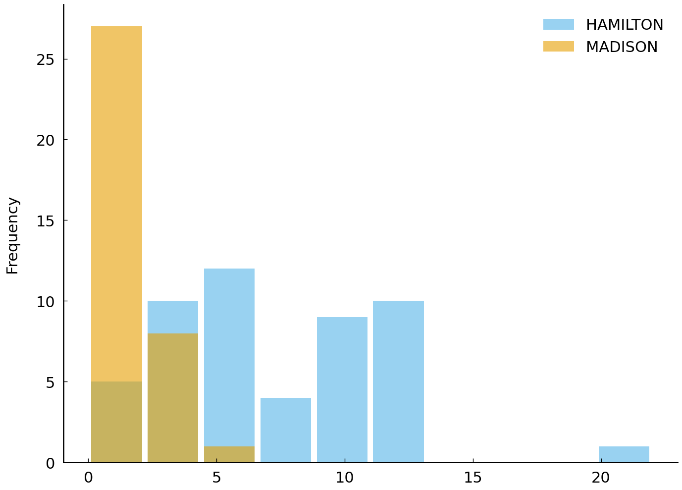
The difference, indeed, is dramatic enough that the visual aid of the histogram is not strictly necessary. Hamilton uses upon far more
than Madison. We can gain a sense of this by comparing any number of summary statistics
(see Statistics Essentials: Who Reads Novels?), including the maximum frequency of upon, the
mean frequency, or the median (50th percentile). These summary statistics are conveniently
produced by the DataFrame method describe():
df_known.groupby('AUTHOR')['upon'].describe()
| count | mean | std | min | 25% | 50% | 75% | max | |
|---|---|---|---|---|---|---|---|---|
| AUTHOR | ||||||||
| HAMILTON | 51.0 | 7.333333 | 4.008325 | 2.0 | 4.0 | 6.0 | 10.00 | 20.0 |
| MADISON | 36.0 | 1.250000 | 1.574348 | 0.0 | 0.0 | 0.5 | 2.25 | 5.0 |
In this particular case, we get an even clearer picture of the difference between the two writers’ use of upon by considering the proportion of essays in which upon appears at all (i.e., one or more times). In our sample, Hamilton always uses upon whereas we are as likely as not to observe it in an essay by Madison.
# The expression below applies `mean` to a sequence of binary observations
# to get a proportion. For example,
# np.mean([False, False, True]) == np.mean([0, 0, 1]) == 1/3
proportions = df_known.groupby('AUTHOR')['upon'].apply(
    lambda upon_counts: (upon_counts > 0).mean())
print(proportions)
AUTHOR
HAMILTON    1.0
MADISON     0.5
Name: upon, dtype: float64
In the preceding block we make use of the methods groupby() (of DataFrame)
and apply() (of SeriesGroupBy)—cf. section
Turnover in naming practices. Recall that the SeriesGroupBy method apply()
works in the following manner: provided a single, callable argument (e.g., a
function or a lambda expression), apply() calls the argument with the discrete
individual series generated by the groupby() method. In this case, apply()
first applies the lambda to the sequence of upon counts associated with
Hamilton and then to the sequence of counts associated with Madison. The
lambda expression itself makes use of a common pattern in scientific
computing: it calculates the average of a sequence of binary (0 or 1)
observations. When the value 1 denotes the presence of a trait and 0 denotes its
absence—as is the case here—the mean will yield the proportion of
observations in which the trait is present. For example, if we were studying the
presence of a specific feature in a set of five essays, we might evaluate
np.mean([0, 0, 1, 1, 0]) and arrive at an answer of \(\frac{2}{5} = 0.4\).
With the heavy lifting behind us, we can create a bar chart which shows the proportion of essays (of known authorship) which contain upon, for each author.
proportions.plot.bar(rot=0);
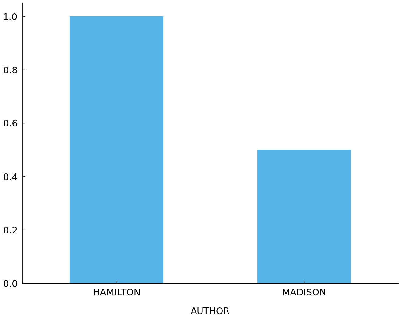
proportions
AUTHOR
HAMILTON    1.0
MADISON     0.5
Name: upon, dtype: float64
Hamilton uses upon more often and more consistently than Madison. While the word upon appears in every one of the 51 essays by Hamilton (100%), the word occurs in only 18 of the 36 essays by Madison (50%). Observing this difference, we should conclude that observing the word upon one or more times in a disputed essay is more consistent with the hypothesis that the author is Hamilton than with the hypothesis that Madison is the author. Precisely how much more consistent is something which must be determined.
Observing the word upon in a disputed essay is hardly decisive evidence that Hamilton wrote the essay; Madison uses the word upon occasionally and, even if he never was observed to have used the word, we need to keep in mind the wide range of unlikely events that could have added an upon to a Madison-authored essay, such as the insertion of an upon by an editor. These considerations will inform a precise description of the probability of the evidence, something we need if we want to use Bayes’s rule and update our belief about the authorship of a disputed essay.
The following is a description of the probability of the evidence (observing the word upon one or more times in a disputed essay) given the hypothesis that Hamilton is the author. Suppose we think that observing upon is far from decisive. Recalling that probabilities are just descriptions of degree of belief (scaled to lie between 0 and 1 and following the axioms of probability), we might say that if Hamilton wrote the disputed essay, the probability of it containing one or more occurrences of the word upon is 0.7. In symbols, we would write \(\Pr(E|H) = 0.7\). We’re using \(\Pr(E|H)\) to denote the probability of observing the word upon in an unobserved essay given that Hamilton is the author.
Now let’s consider Madison. Looking at how often Madison uses the word upon, we anticipate that it is as likely as not that he will use the word (one or more times) if the disputed essay is indeed written by him. Setting \(\Pr(E|\neg H) = 0.5\) seems reasonable. Suppose that we are now presented with one of the disputed essays and we observe that the word upon does indeed occur one or more times. Bayes’s rule tells us how our belief should change after observing this piece of evidence:
Since the hypothesis space is partitioned by \(H\) and \(\neg H\) (“not H”), the formula can be rewritten. As we only have two possible authors (Hamilton or Madison) we can write \(H\) for the hypothesis that Hamilton wrote the disputed essay and \(\neg H\) for the hypothesis that Madison (i.e., not Hamilton) wrote the disputed essay. And since we have settled on values for all the terms on the right-hand side of the equation we can complete the calculation:
It makes sense that our degree of belief in Hamilton being the author increases from 0.5 to 0.58 in this case: Hamilton uses upon far more than Madison, so seeing this word in a disputed essay should increase (or, at least, certainly not decrease) the plausibility of the claim that Hamilton is the author. The precise degree to which it changes is what Bayes’s rule contributes.
Random variables and probability distributions#
In the previous example, we simplified the analysis by only concerning ourselves with whether or not a word occurred one or more times. In this specific case the simplification was not consequential, since we were dealing with a case where the presence or absence of a word was distinctive. Assessing the distinctiveness of word usage in cases where the word is common (i.e., it typically occurs at least once) requires the use of a discrete probability distribution. One distribution which will allow us to model the difference with which authors use words such as by and whilst is the negative binomial distribution. When working with models of individual word frequencies in text documents, the negative binomial distribution is almost always a better choice than the binomial distribution.
The key feature of texts that the negative binomial distribution captures and that the binomial distribution does not is the burstiness or contagiousness of uncommon words: if an uncommon word, such as a location name or person’s name, appears in a document, the probability of seeing the word a second time should go up [Church and Gale, 1995].
Examining the frequency with which Madison and Hamilton use the word by, it is easy to detect a pattern. Based on the sample we have, Madison reliably uses the word by more often than Hamilton does: Madison typically uses the word 13 times per 1,000 words; Hamilton typically uses it about 6 times per 1,000 words. To reproduce these rate calculations, we first scale all word frequency observations into rate per 1,000 words. After doing this, we exclude essays not written by Hamilton or Madison and then display the average rate of by.
df = pd.read_csv('data/federalist-papers.csv', index_col=0)
author = df['AUTHOR']  # save a copy of the author column
df = df.drop('AUTHOR', axis=1)  # remove the author column
df = df.divide(df.sum(axis=0))  # rate per 1 word
df *= 1000  # transform from rate per 1 word to rate per 1,000 words
df = df.round()  # round to nearest integer
df['AUTHOR'] = author  # put author column back
df_known = df[df['AUTHOR'].isin({'HAMILTON', 'MADISON'})]

df_known.groupby('AUTHOR')['by'].describe()
| count | mean | std | min | 25% | 50% | 75% | max | |
|---|---|---|---|---|---|---|---|---|
| AUTHOR | ||||||||
| HAMILTON | 51.0 | 7.019608 | 4.925404 | 1.0 | 5.0 | 6.0 | 9.0 | 34.0 |
| MADISON | 36.0 | 12.916667 | 4.094421 | 5.0 | 10.0 | 12.5 | 15.0 | 23.0 |
We can visualize the difference in the authors’ use of by with two overlapping histograms:
df_known.groupby('AUTHOR')['by'].plot.hist(
    alpha=0.6, range=(0, 35), rwidth=0.9, legend=True);
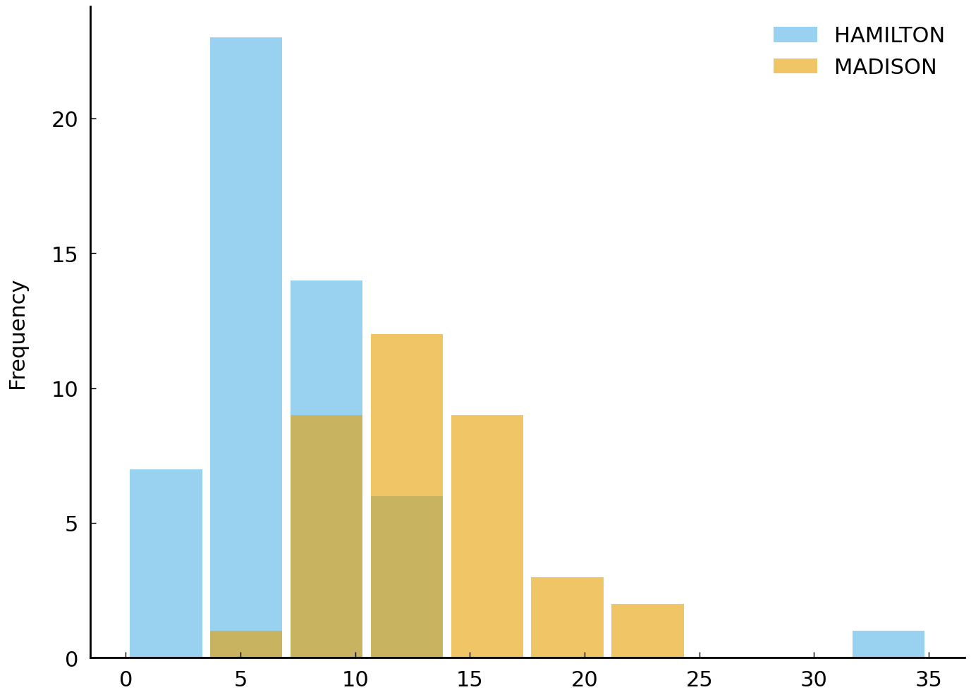
Looking at the distribution of frequencies above, it is clear that there is evidence of a systematic difference in the rate the two writers use the word by. A high rate of by for Hamilton (the 75th percentile is 12) is less than the typical rate Madison uses the word (the median for Madison is 12.5).
There is one case, Federalist No. 83, clearly visible in the histogram, which
is written by Hamilton and features a very high rate of by. This high rate has
a simple explanation. Federalist No. 83’s topic is the institution of trial
by jury and understandably features the two-word sequence by jury 36
times. If we ignore the by instances which occur in the sequence by jury,
by occurs about 7 times per 1,000 words, safely in the region of expected
rates from Hamilton given the other texts. Federalist No. 83 provides an
excellent cautionary example of an allegedly content-free “function word” by
turning out to be intimately connected to the content of a text. We can verify
that the outlier is indeed Federalist No. 83 by querying our DataFrame:
print(df_known.loc[df_known['by'] > 30, 'by'])
83    34.0
Name: by, dtype: float64
And we can verify, using the full text of Federalist No. 83, that the two-word phrase by jury appears 36 times in the text. Setting these appearances aside, we can further check that the rate of by (without by jury) is about 7 per 1,000 words.
with open('data/federalist-83.txt') as infile:
    text = infile.read()

# a regular expression here would be more robust
by_jury_count = text.count(' by jury')
by_count = text.count(' by ')
word_count = len(text.split())  # crude word count
by_rate = 1000 * (by_count - by_jury_count) / word_count

print('In Federalist No. 83 (by Hamilton), without "by jury", '
      f'"by" occurs {by_rate:.0f} times per 1,000 words on average.')
In Federalist No. 83 (by Hamilton), without "by jury", "by" occurs 7 times per 1,000 words on average.
In the block above, we read in a file containing the text of Federalist No. 83 and count the number of times by jury occurs and the number of times by (without jury) occurs. We then normalize the count of by (without jury) to the rate per 1,000 words for comparison with the rate observed elsewhere.
While it would be convenient to adopt the approach we took with upon and apply it to the present case, unfortunately we cannot. The word by appears in every one of the essays with an established author; the approach we used earlier will not work. That is, if we expect both authors to use by at least once per 1,000 words, the probability of the author being Hamilton given that by occurs at least once is very high and the probability of the author being Madison given that by occurs at least once is also very high. In such a situation—when \(\Pr(E|H) \approx \Pr(E|\neg H)\)—Bayes’s rule guarantees we will learn little: \(\Pr(H|E) \approx P(H)\). In order to make use of information about the frequency of by in the unknown essay, we need a more nuanced model of each author’s tendency to use by. We need to have a precise answer to questions such as the following: if we pick 1,000 words at random from Madison’s writing, how likely are we to find 6 instances of by among them? More than 12 instances? How surprising would it be to find 40 or more?
Negative binomial distribution#
We need a model expressive enough to answer all these questions. This model must be capable of saying that among 1,000 words chosen at random from the known essays by an author, the probability of finding \(x\) instances of by is a specific probability. In symbols we would use the symbol \(X\) to denote the “experiment” of drawing 1,000 words at random from an essay and reporting the number of by instances and write lowercase \(x\) for a specific realization of the experiment. This lets us write \(p = \Pr(X = x|H) = f(x)\) to indicate the probability of observing a rate of \(x\) by tokens per 1,000 words given that the text is written by Hamilton. Whatever function, \(f\), we choose to model \(X\) (called a random variable), we will need it to respect the axioms of probability. For example, following axiom 1, it must not report a probability less than zero or greater than 1. There are many functions (called “probability mass functions”) which will do the job. Some will be more faithful than others in capturing the variability of rates of by which we observe (or feel confident we will observe). That is, some will be better aligned with our degrees of belief in observing the relevant rate of by given that Hamilton is the author. Candidate distributions include the Poisson distribution, the binomial distribution, and the negative binomial distribution. We will follow Mosteller and Wallace and use the negative binomial distribution.
\(X\), a random variable, is said to be distributed according to a negative binomial distribution with parameters \(\alpha\) and \(\beta\) if
Random variable
A random variable is defined as a function from a sample space into the real numbers. A random variable, \(X\), intended to represent whether the toss of a coin landed “heads” would be associated with the sample space \(S = \{H, T\}\), where \(H\) and \(T\) indicate the two possible outcomes of the toss (\(H\) for “heads” and \(T\) for “tails”). Each of these potential outcomes is associated with a probability. In this case, \(\Pr(H)\) and \(\Pr(T)\) might be equal to 0.5. The random variable \(X\) takes on numeric values; here it would take on the value 1 if the outcome of the random experiment (i.e., “flipping a coin”) was \(H\), otherwise the random variable would take on the value 0. That is, we observe \(X = 1\) if and only if the outcome of the random experiment is \(H\). The probability function \(\Pr\) associated with the sample space induces a probability function associated with \(X\) which we could write \(\Pr_X\). This function must satisfy the axioms of probability. In symbols, it would be written \(\Pr_X(X = x_i) = \Pr(\{s_j \in S : X(s_j) = x_i\})\) (Casella and Berger [2001], section 1.1-1.4).
This function \(\Pr(X = x \,|\, \alpha, \beta)\) is a probability mass function (abbreviated “pmf”). If a random variable follows this distribution we may also write \(X \sim \distro{NegBinom}(\alpha,\beta)\) and say that \(X\) is distributed according to a negative binomial distribution.
Given a sequence of draws from such a random variable, we would find that the sequence has mean \(\frac{\alpha}{\beta}\) and variance \(\frac{\alpha}{\beta^2} (\beta + 1)\). The derivation of these results from the negative binomial pmf above is a subject covered in most probability courses and introductory textbooks.
For example, if \(X \sim \distro{NegBinom}(5, 1)\) then the probability of
observing \(X = 6\) is, according to the pmf above, approximately 10 percent. The
probability of observing \(X = 14\) is considerably lower, 0.5 percent. We can
verify these calculations by translating the negative binomial pmf stated above
into Python code. The following function, negbinom_pmf(), makes use of one
possibly unfamiliar function, scipy.special.binom(a, b) which calculates,
as the name suggests, the binomial coefficient \(\binom{a}{b}\).
import scipy.special

def negbinom_pmf(x, alpha, beta):
    """Negative binomial probability mass function."""
    # In practice this calculation should be performed on the log
    # scale to reduce the risk of numeric underflow.
    return (
        scipy.special.binom(x + alpha - 1, alpha - 1)
        * (beta / (beta + 1)) ** alpha
        * (1 / (beta + 1)) ** x
    )

print('Pr(X = 6):', negbinom_pmf(6, alpha=5, beta=1))
print('Pr(X = 14):', negbinom_pmf(14, alpha=5, beta=1))
Pr(X = 6): 0.1025390625
Pr(X = 14): 0.00583648681640625
Further discussion of discrete distributions and probability mass functions is not necessary to appreciate the immediate usefulness of the negative binomial distribution as a tool which provides answers to the questions asked above. With suitably chosen parameters \(\alpha\) and \(\beta\), the negative binomial distribution (and its associated probability mass function) provides precise answers to questions having the form we are interested in, questions such as the following: how likely is it for a 1,000-word essay by Hamilton to contain 6 instances of by? Moreover, the negative binomial distribution can provide plausible answers to such questions, where plausibility is defined with reference to our degrees of belief.
How well the answers align with our beliefs about plausible rates of by depends on the choice of the parameters \(\alpha\) and \(\beta\). It is not difficult to find appropriate parameters, as the graphs below will make clear. The graphs show the observed rates of by from Hamilton’s essays alongside simulated rates drawn from negative binomial distributions with three different parameter settings. How we arrived at these precise parameter settings is addressed in the Appendix Fitting a negative binomial distribution.
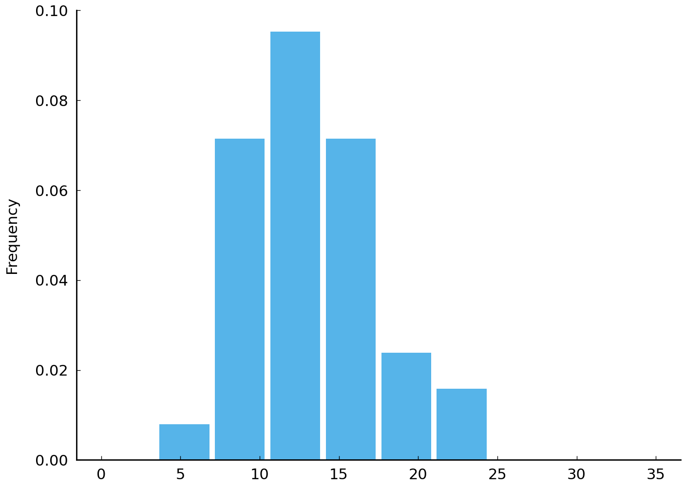
The first plot bewlow will show the empirical distribution of the by rates we observe in Hamilton’s (non-disputed) essays. These observed rates are all the information we have about Hamilton’s tendency to use by, so we will choose a negative binomial distribution which roughly expresses the same information.
df_known[df_known['AUTHOR'] == 'HAMILTON']['by'].plot.hist(
    range=(0, 35), density=True, rwidth=0.9);
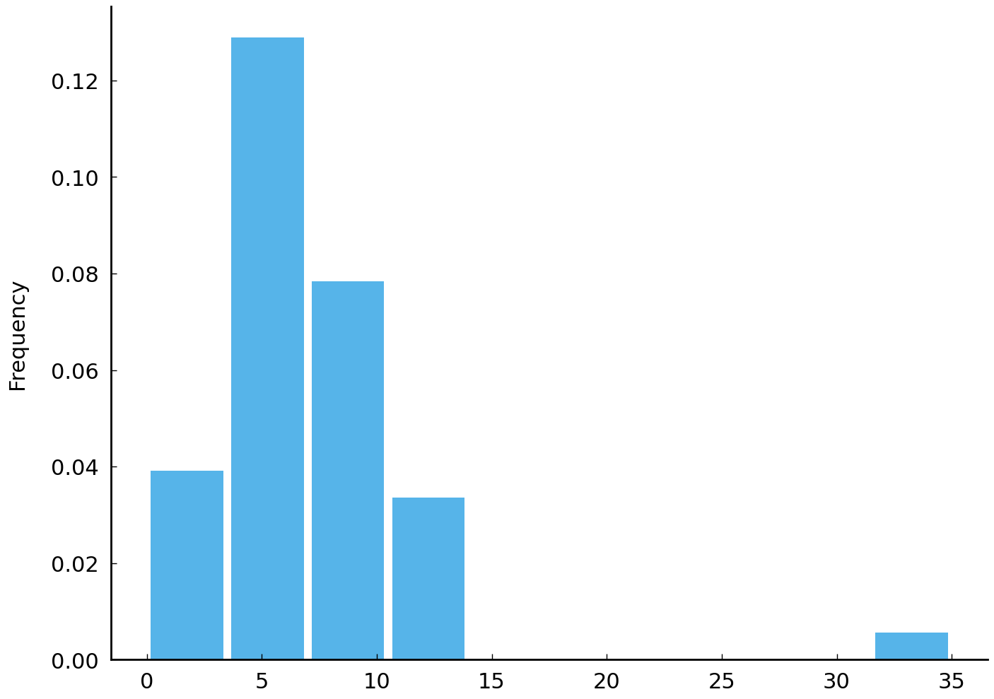
df_known[df_known['AUTHOR'] == 'HAMILTON']['by'].describe()
count    51.000000
mean      7.019608
std       4.925404
min       1.000000
25%       5.000000
50%       6.000000
75%       9.000000
max      34.000000
Name: by, dtype: float64
Now that we know what we’re looking for – a distribution with plenty of mass between 1 and 10 and minimal support for observations greater than 40 – we can look at various negative binomial distributions and see if any will work as approximations of our degrees of belief about Hamilton’s tendency to use by around 1787.
import itertools
import matplotlib.pyplot as plt

x = np.arange(60)
alphas, betas = [5, 6.5, 12, 16], [1.5, 0.5, 0.7]
params = list(itertools.product(alphas, betas))
pmfs = [negbinom_pmf(x, alpha, beta) for alpha, beta in params]

fig, axes = plt.subplots(4, 3, sharey=True, figsize=(10, 8))
axes = axes.flatten()

for ax, pmf, (alpha, beta) in zip(axes, pmfs, params):
    ax.bar(x, pmf)
    ax.set_title(fr'$\alpha$ = {alpha}, $\beta$ = {beta}')
plt.tight_layout();
findfont: Font family ['sans-serif'] not found. Falling back to DejaVu Sans.
findfont: Generic family 'sans-serif' not found because none of the following families were found: "Roboto Condensed Regular"
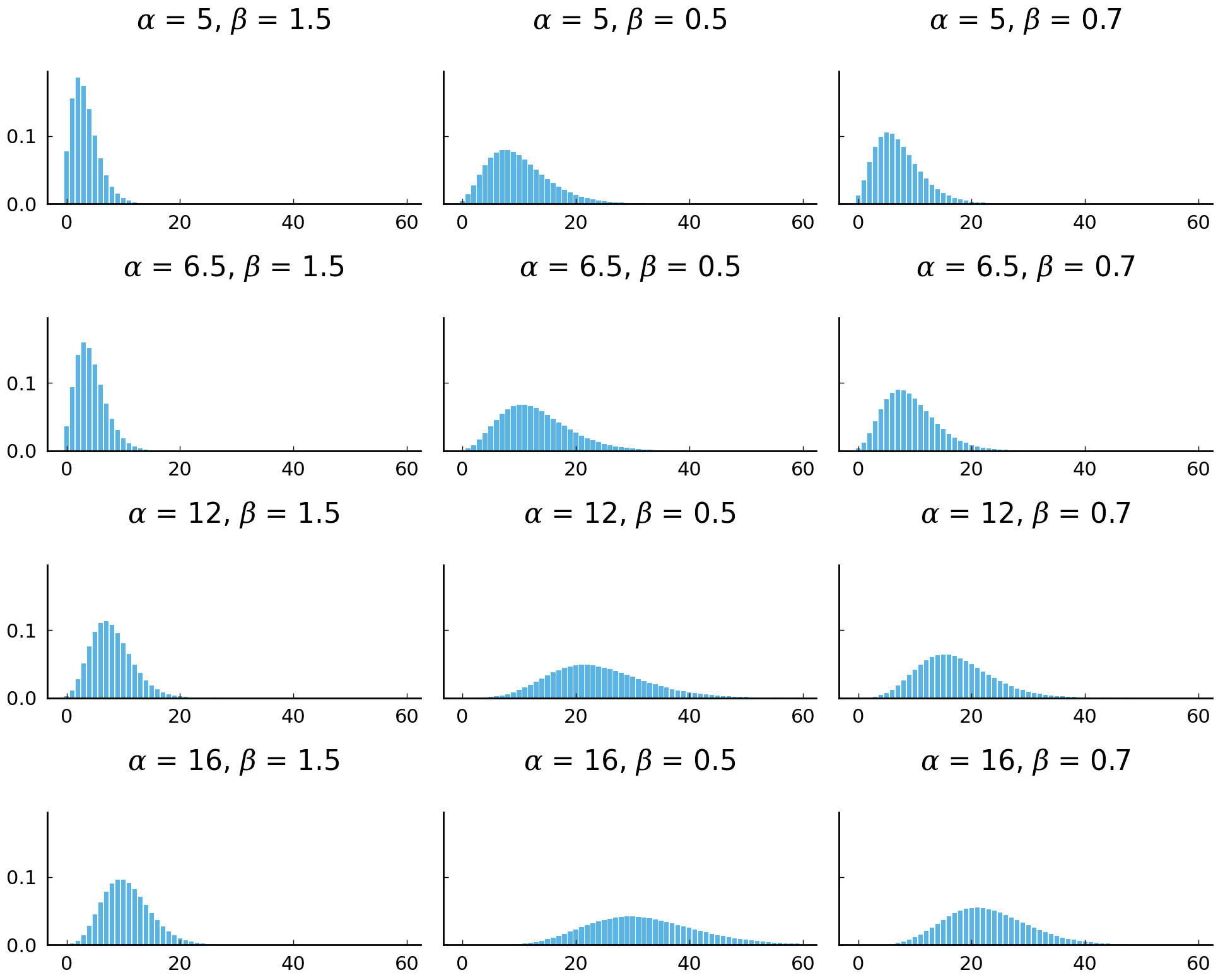
The parameterization of \(\alpha = 5\) and \(\beta = 0.7\) is one of the models that (visually) resembles the empirical distribution. Indeed, if we accept \(\distro{NegBinom}(5, 0.7)\) as modeling our degrees of belief about Hamilton’s use of by, the distribution has the attractive feature of predicting the same average rate of by as we observe in the Hamilton essays in the corpus. We can verify this by simulating draws from the distribution and comparing the summary statistics of our sampled values with the observations we have encountered so far.
def negbinom(alpha, beta, size=None):
    """Sample from a negative binomial distribution.

    Uses `np.random.negative_binomial`, which makes use of a
    different parameterization than the one used in the text.
    """
    n = alpha
    p = beta / (beta + 1)
    return np.random.negative_binomial(n, p, size)

samples = negbinom(5, 0.7, 10000)
# put samples in a pandas Series in order to calculate summary statistics
pd.Series(samples).describe()
count    10000.00000
mean         7.07620
std          4.11972
min          0.00000
25%          4.00000
50%          6.00000
75%          9.00000
max         29.00000
dtype: float64
The negative binomial distribution with fixed
parameters—\(\alpha = 5\) and \(\beta = 0.7\) were used in the code block above—is an
oracle which answers the questions we have. For any observed value of the rate of by in
a disputed essay we can provide an answer to the question, “Given that Hamilton is the
author of the disputed essay, what is the probability of observing a rate \(x\) of by?”
The answer is \(\Pr(X = x|\alpha, \beta)\) for fixed values of \(\alpha\) and \(\beta\),
something we can calculate directly with the function negbinom_pmf(x, alpha, beta).
Now that we have a way of calculating the probability of by under the hypothesis that
Hamilton is the author, we can calculate a quantity that plays the same role that
\(\Pr(E|H)\) played in the previous section. This will allow us to use Bayes’s rule to calculate our degree of belief in the claim that
Hamilton wrote a disputed essay, given an observed rate of by in the essay.
Now let us consider some plausible models of Madison’s use of the word by. In order to use Bayes’s rule we will need to be able to characterize how plausible different rates of by are, given that Madison is the author.
df_known[df_known['AUTHOR'] == 'MADISON']['by'].plot.hist(
    density=True, rwidth=0.9, range=(0, 35)  # same scale as with Hamilton
);
x = np.arange(60)
alphas, betas = [100, 50, 28, 10], [23, 4, 1.3]
params = list(itertools.product(alphas, betas))
pmfs = [negbinom_pmf(x, alpha, beta) for alpha, beta in params]

fig, axes = plt.subplots(4, 3, sharey=True, figsize=(10, 8))
axes = axes.flatten()

for ax, pmf, (alpha, beta) in zip(axes, pmfs, params):
    ax.bar(x, pmf)
    ax.set_title(fr'$\alpha$ = {alpha}, $\beta$ = {beta}')
plt.tight_layout()
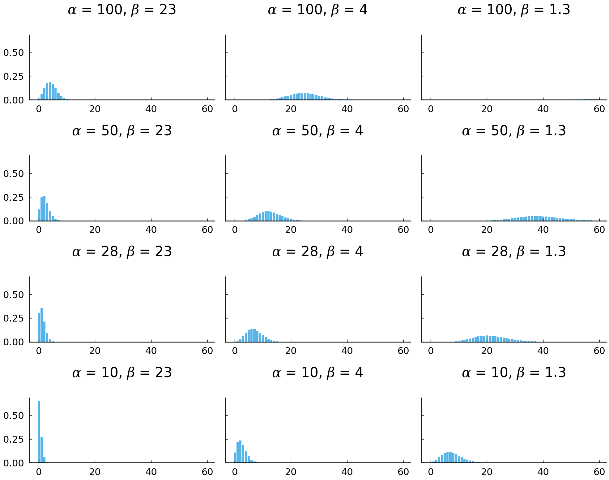
If \(\alpha\) is 50 and \(\beta\) is 4, the model resembles the empirical distribution of the rates of by in the Madison essays. Most values are between 5 and 25 and the theoretical mean of the negative binomial distribution is similar to the empirical mean. Compare the two (idealized) models of the use of by with the rates of by we have observed in the essays with known authorship.
authors = ('HAMILTON', 'MADISON')
alpha_hamilton, beta_hamilton = 5, 0.7
alpha_madison, beta_madison = 50, 4

# observed
fig, axes = plt.subplots(2, 1, sharex=True, sharey=True)
df_known.groupby('AUTHOR')['by'].plot.hist(
    ax=axes[0], density=True, range=(0, 35), rwidth=0.9, alpha=0.6,
    title='Hamilton v. Madison (observed)', legend=True)

# model
simulations = 10000
for author, (alpha, beta) in zip(authors, [(alpha_hamilton, beta_hamilton),
                                           (alpha_madison, beta_madison)]):
    pd.Series(negbinom(alpha, beta, size=simulations)).plot.hist(
        label=author, density=True, rwidth=0.9, alpha=0.6, range=(0, 35), ax=axes[1])
axes[1].set_xlim((0, 40))
axes[1].set_title('Hamilton v. Madison (model)')
axes[1].legend()
plt.tight_layout();
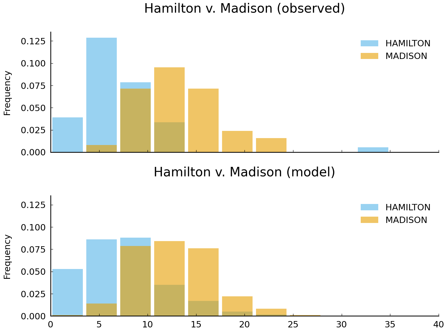
With the negative binomial distribution available as a rough model for our beliefs about each author’s use of by, we have all that is required to use Bayes’s rule and assess how observing a given rate of by in a disputed essay should persuade us of the plausibility of Hamilton or Madison being the author.
Imagine we are presented with one of the disputed essays and observe that
the word by occurs 14 times per 1,000 words—the rate observed, in fact, in
No. 57. A casual inspection of the rates for essays with known authorship tells
us that 14 instances of by would be rather high for Hamilton (9 per 1,000 on
average in our samples); 14 is closer to the expected rate for Madison. So we
should anticipate that the calculation suggested by Bayes’ rule would increase
the odds favoring Madison. Using \(\Pr(H) = \Pr(\neg H) = 0.5\) as before, we use
the probability mass function for the negative binomial distribution to
calculate the probability of observing a rate of 14 per 1,000 in an essay
authored by Hamilton and the probability of observing a rate of 14 per 1,000 in
an essay authored by Madison (probabilities analogous to \(\Pr(E|H)\) and \(\Pr(E|\neg H)\) in the
previous section). Instead of \(E\) we will write \(X\) for the observed rate of
by. So \(\Pr(X = 14|H) = \Pr(X = x|\alpha_{Hamilton},\beta_{Hamilton}) = 0.022\) and
\(\Pr(X = 14|\neg H) = \Pr(X = x|\alpha_{Madison}, \beta_{Madison}) = 0.087\). The way
we find these values is to use the function negbinom_pmf(), which we defined
above.
likelihood_hamilton = negbinom_pmf(14, alpha_hamilton, beta_hamilton)
print(likelihood_hamilton)
0.021512065936254765
likelihood_madison = negbinom_pmf(14, alpha_madison, beta_madison)
print(likelihood_madison)
0.08742647980678281
pr_hamilton = likelihood_hamilton * 0.5 / (likelihood_hamilton * 0.5 + likelihood_madison * 0.5)
print(pr_hamilton)
0.19746973662561154
In the code above we’ve used the term likelihood to refer to the probability of the evidence given the hypothesis, \(\Pr(E|H)\).
Bayes’s rule tells us how to update our beliefs about whether or not Hamilton wrote this hypothesized disputed essay about which we have only learned the rate of by instances is 14 per 1,000. In such a case the odds turn against Hamilton being the author, approximately 4 to 1 in favor of Madison. The rate of by in the unknown essay is just one piece of evidence which we might consider in assessing how much plausibility we assign to the claim “Hamilton wrote paper No. 52”. Mosteller and Wallace consider the rates of 30 words (by is in the group of “final words”) in their analysis (Mosteller and Wallace [1964], 67–68).
Further Reading#
This chapter introduced Bayesian inference, one technique for learning from experience. Among many possible approaches to learning from observation, Bayesian inference provides a specific recipe for using probabilities to describe degrees of belief and for updating degrees of belief based on observation. Another attractive feature of Bayesian inference is its generality. Provided we can come up with a description of our prior degree of belief in an event occurring, as well as a description of how probable some observation would be under various hypotheses about the event, Bayes’s rule provides us with a recipe for updating our degree of belief in the event being realized after taking into consideration the observation. To recall the example that we concluded with, Bayesian inference provides us with a principled way of arriving at the claim that “it is very likely that Madison (rather than Hamilton) wrote Federalist No. 62” given observed rates of word usage in Federalist No. 62. This is a claim that historians writing before 1950 had no way of substantiating. Thanks to Bayesian inference and the work of Mosteller and Wallace, the evidence and procedure supporting this claim are accessible to everyone interested in this case of disputed authorship.
For essential background reading related to this chapter, we recommend Grinstead and Snell [2012] which provides an introduction to discrete and continuous probability. Their book is published by the American Mathematical Society and is available online at. For those interested in further reading related to the topics addressed in this chapter, we recommend an introductory text on Bayesian inference. Those with fluency in single-variable calculus and probability will be well served by Hoff [2009]. While Hoff [2009] uses the R programming language for performing computation and visualizing results, the code provided may be translated into Python without much effort.
Excercises#
Easy#
Which of the following terms is used to denote a prior belief? a) \(\Pr(E|H)\), b) \(\Pr(H|E)\), or c) \(\Pr(H)\).
Which of the following terms is used to describe the likelihood of an observation given a hypothesis? a) \(\Pr(E|H)\), b) \(\Pr(E)\), or c) \(\Pr(H|E)\).
Recall the example about Pynchon from the introduction to this chapter. Suppose we improve our stylometric test to accurately identify a novel as being written by Pynchon from 90 percent to 99 percent of the time. The false positive rate also decreased and now equals 0.1 percent. The probability that a novel was written by Pynchon is still 0.001 percent. Suppose another text tests positive on our stylometric test. What is the probability that the text was written by Pynchon?
Mosteller and Wallace describe Madison’s and Hamilton’s word usage in terms of frequency per 1,000 words. While most essays were longer—typically between 2,000 and 3,000 words—pretending as if each document were 1,000 words and contained a fixed number of occurrences of the words of interest allows us to compare texts of different lengths. Inaccuracies introduced by rounding will not be consequential in this case. Calculate the frequency per 1,000 words of upon, the, and enough.
Moderate#
Mosteller and Wallace started their investigation of the authorship of the disputed essays in The Federalist Papers by focusing on a handful of words, which, closely reading the essays, had revealed as distinctive: while, whilst, upon, enough. Focus on the word enough. Suppose you are about to inspect one of the disputed essays and see if enough appears.
How many times does the word enough occur at least once in essays by Madison? How many times does the word occur at least once in essays by Hamilton?
Establish values for \(\Pr(H)\), \(\Pr(E|H)\), and \(\Pr(E|\neg H)\) that you find credible. (\(\Pr(E|H)\) here is the probability that the word enough appears in a disputed essay when Hamilton, rather than Madison, is the author.)
Suppose you learn that enough appears in the disputed essay. How does your belief about the author change?
Challenging#
Consider the rate at which the word of occurs in texts with known authorship. If you were to use a binomial distribution (not a negative binomial distribution) to model each author’s use of the word of (expressed in frequency per 1,000 words), what value would you give to the parameter \(\theta\) associated with Hamilton? And with Madison?
Working with the parameter values chosen above, suppose you observe a disputed essay with a rate of 8 ofs per 1,000 words. Does this count as evidence in favor of Madison being the author or as evidence in favor of Hamilton being the author?
Appendix#
Bayes’s rule#
In order to derive Bayes’s rule we first begin with the third axiom of probability:
If we let \(C\) be an event which encompasses all possible events (\(A \and C = A\)) we have a simpler statement about a conditional probability:
Replacing \(A\) and \(B\) with \(H_j\) and \(E\), respectively, we arrive at an initial form of Bayes’s rule:
The denominator, \(\Pr(E)\) may be unpacked by using the rule of marginal probability:
Replacing \(\Pr(E)\) in the initial statement we have the final, familiar form of Bayes’s rule:
Fitting a negative binomial distribution#
Finding values for \(\alpha\) and \(\beta\) which maximize the sampling probability (as a function of \(\alpha\) and \(\beta\)) is tricky. Given knowledge of the sample mean \(\bar x\) and the value of \(\alpha\), the value of \(\beta\) which maximizes the sampling probability (as a function of \(\beta\)) can be found by finding the critical points of the function. (The answer is \(\hat \beta = \frac{\alpha}{\bar x}\) and the derivation is left as an exercise for the reader.) Finding a good value for \(\alpha\) is challenging. The path of least resistance here is numerical optimization. Fortunately, the package SciPy comes with a general purpose function for optimization which tends to be reliable and requires minimal configuration:
# `x` is a sample of Hamilton's rates of 'by' (per 1,000 words)
x = np.array([13, 6, 4, 8, 16, 9, 10, 7, 18, 10, 7, 5, 8, 5, 6, 14, 47])
pd.Series(x).describe()
count    17.000000
mean     11.352941
std      10.024602
min       4.000000
25%       6.000000
50%       8.000000
75%      13.000000
max      47.000000
dtype: float64
import scipy.optimize
import scipy.special

# The function `negbinom_pmf` is defined in the text.


def estimate_negbinom(x):
    """Estimate the parameters of a negative binomial distribution.

    Maximum-likelihood estimates of the parameters are calculated.
    """
    def objective(x, alpha):
        beta = alpha / np.mean(x)  # MLE for beta has closed-form solution
        return -1 * np.sum(np.log(negbinom_pmf(x, alpha, beta)))
    alpha = scipy.optimize.minimize(
        lambda alpha: objective(x, alpha), x0=np.mean(x), bounds=[(0, None)], tol=1e-7).x[0]
    return alpha, alpha / np.mean(x)


alpha, beta = estimate_negbinom(x)
print(alpha, beta)
2.9622164213528452 0.260920617424862
/var/folders/s8/1h01d3xx303c51_q78_b9gjw0000gn/T/ipykernel_48099/183489177.py:14: RuntimeWarning: divide by zero encountered in log
  return -1 * np.sum(np.log(negbinom_pmf(x, alpha, beta)))